
A tidyverse suite for (pre-) machine-learning: cluster, PCA, permute, impute, rotate, redundancy, triangular, smart-subset, abundant and variable features.
This repository is no longer maintained and superseeded by tidybulk ================
It tidies up your playground\!

Please have a look also to
- tidygate for adding custom gate information to your tibble - tidyHeatmap for heatmaps produced with tidy principles - tidybulk brings transcriptomics to the tidyverse
Functions/utilities available
It does a lot\! cluster, PCA, permute, impute, rotate, redundancy-removal, triangular, smart-subset, identify abundant and variable features.
| Function | Description | | ------------------- | ----------------------------------------------------------------------- | | reduce_dimensions | Perform dimensionality reduction (PCA, MDS, tSNE) | | rotate_dimensions | Rotate two dimensions of a degree | | cluster_elements | Labels elements with cluster identity | | remove_redundancy | Filter out elements with highly correlated features | | fill_missing | Fill values of missing element/feature pairs | | impute_missing | Impute values of missing element/feature pairs | | permute_nest | From one column build a two permuted columns with nested information | | combine_nest | From one column build a two combination columns with nested information | | keep_variable | Keep top variable features | | lower_triangular | keep rows corresponding to a lower triangular matrix |
| Utilities | Description | | ----------- | ---------------------------------------------------------------- | | as_matrix | Robustly convert a tibble to matrix | | subset | Select columns with information relative to a column of interest |
Minimal input data frame
| element | feature | value | | --------------- | --------------- | --------- | | chr or fctr | chr or fctr | numeric |
Output data frame
| element | feature | value | new information | | --------------- | --------------- | --------- | --------------- | | chr or fctr | chr or fctr | numeric | … |
Installation
r
devtools::install_github("stemangiola/nanny")
Introduction
nanny is a collection of wrapper functions for high level data analysis and manipulation following the tidy paradigm.
Tidy data
r
mtcars_tidy =
    mtcars %>%
    astibble(rownames="carmodel") %>%
    mutateat(vars(-carmodel,- hp, -vs), scale) %>%
    gather(feature, value, -car_model, -hp, -vs)
mtcars_tidy
## # A tibble: 288 x 5 ## car_model hp vs feature value ##
reduce_dimensions
We may want to reduce the dimensions of our data, for example using PCA, MDS of tSNE algorithms. reduce_dimensions takes a tibble, column names (as symbols; for element, feature and value) and a method (e.g., MDS, PCA or tSNE) as arguments and returns a tibble with additional columns for the reduced dimensions.
MDS
r
mtcarstidyMDS =
  mtcars_tidy %>%
  reducedimensions(carmodel, feature, value, method="MDS", .dims = 3)
On the x and y axes axis we have the reduced dimensions 1 to 3, data is coloured by cell type.
r
mtcarstidyMDS %>% subset(car_model)  %>% select(contains("Dim"), everything())
## # A tibble: 32 x 6 ## Dim1 Dim2 Dim3 car_model hp vs ##
r
mtcarstidyMDS %>%
    subset(car_model) %>%
  GGally::ggpairs(columns = 4:6, ggplot2::aes(colour=factor(vs)))
PCA
r
mtcarstidyPCA =
  mtcars_tidy %>%
  reducedimensions(carmodel, feature, value, method="PCA", .dims = 3)
On the x and y axes axis we have the reduced dimensions 1 to 3, data is coloured by cell type.
r
mtcarstidyPCA %>% subset(car_model) %>% select(contains("PC"), everything())
## # A tibble: 32 x 6 ## PC1 PC2 PC3 car_model hp vs ##
r
mtcarstidyPCA %>%
     subset(car_model) %>%
  GGally::ggpairs(columns = 4:6, ggplot2::aes(colour=factor(vs)))
tSNE
r
mtcarstidytSNE =
    mtcars_tidy %>%
    reducedimensions(carmodel, feature, value, method = "tSNE")
Plot
r
mtcarstidytSNE %>%
    subset(car_model) %>%
    select(contains("tSNE"), everything())
## # A tibble: 32 x 5 ## tSNE1 tSNE2 car_model hp vs ##
r
mtcarstidytSNE %>%
    subset(car_model) %>%
    ggplot(aes(x = tSNE1, y = tSNE2, color=factor(vs))) + geompoint() + mytheme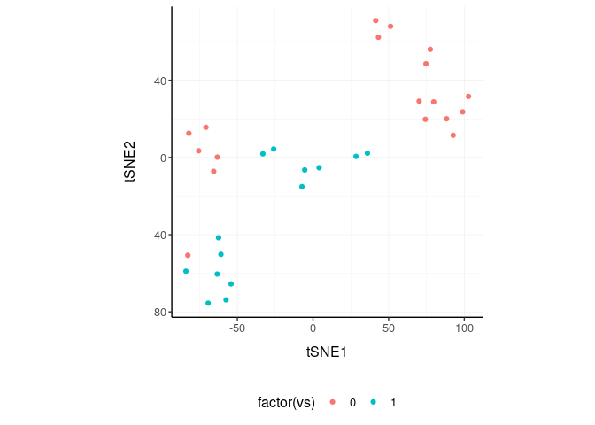
rotate_dimensions
We may want to rotate the reduced dimensions (or any two numeric columns really) of our data, of a set angle. rotate_dimensions takes a tibble, column names (as symbols; for element, feature and value) and an angle as arguments and returns a tibble with additional columns for the rotated dimensions. The rotated dimensions will be added to the original data set as <NAME OF DIMENSION> rotated <ANGLE> by default, or as specified in the input arguments.
r
mtcarstidyMDS.rotated =
  mtcarstidyMDS %>%
    rotatedimensions(Dim1, Dim2, .element = carmodel, rotation_degrees = 45, action="get")
Original On the x and y axes axis we have the first two reduced dimensions, data is coloured by cell type.
r
mtcarstidyMDS.rotated %>%
    ggplot(aes(x=Dim1, y=Dim2, color=factor(vs) )) +
  geom_point() +
  my_theme
Rotated On the x and y axes axis we have the first two reduced dimensions rotated of 45 degrees, data is coloured by cell type.
r
mtcarstidyMDS.rotated %>%
    ggplot(aes(x=Dim1 rotated 45, y=Dim2 rotated 45, color=factor(vs) )) +
  geom_point() +
  my_theme
cluster_elements
We may want to cluster our data (e.g., using k-means element-wise). cluster_elements takes as arguments a tibble, column names (as symbols; for element, feature and value) and returns a tibble with additional columns for the cluster annotation. At the moment only k-means clustering is supported, the plan is to introduce more clustering methods.
k-means
r
mtcarstidycluster = mtcarstidyMDS %>%
  clusterelements(carmodel, feature, value, method="kmeans",  centers = 2, action="get" )
We can add cluster annotation to the MDS dimension reduced data set and plot.
r
 mtcarstidycluster %>%
    ggplot(aes(x=Dim1, y=Dim2, color=cluster_kmeans)) +
  geom_point() +
  my_theme
SNN
r
mtcarstidySNN =
    mtcarstidytSNE %>%
    clusterelements(carmodel, feature, value, method = "SNN")
We can add cluster annotation to the tSNE dimension reduced data set and plot.
r
mtcarstidySNN %>%
    subset(car_model) %>%
    select(contains("tSNE"), everything())
## # A tibble: 32 x 6 ## tSNE1 tSNE2 carmodel hp vs clusterSNN ##
r
mtcarstidySNN %>%
    subset(car_model) %>%
    ggplot(aes(x = tSNE1, y = tSNE2, color=clusterSNN)) + geompoint() + my_theme
gating
r
mtcarstidyMDS %>%
    clusterelements(carmodel, c(Dim1, Dim2), method="gate", .color=group)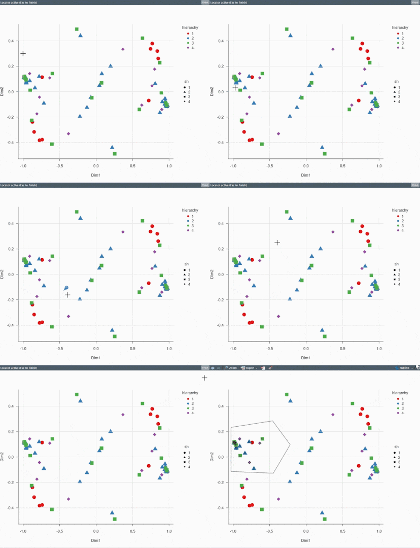
## # A tibble: 288 x 9 ## car_model hp vs feature value Dim1 Dim2 Dim3 gate ##
drop_redundant
We may want to remove redundant elements from the original data set (e.g., elements or features), for example if we want to define cell-type specific signatures with low element redundancy. remove_redundancy takes as arguments a tibble, column names (as symbols; for element, feature and value) and returns a tibble dropped recundant elements (e.g., elements). Two redundancy estimation approaches are supported:
removal of highly correlated clusters of elements (keeping a representative) with method=“correlation”
r
mtcarstidynon_redundant =
    mtcarstidyMDS %>%
  removeredundancy(carmodel, feature, value)
We can visualise how the reduced redundancy with the reduced dimentions look like
r
mtcarstidynon_redundant %>%
    subset(car_model) %>%
    ggplot(aes(x=Dim1, y=Dim2, color=factor(vs))) +
  geom_point() +
  my_theme
fill_missing
This function allows to obtain a rectangular underlying data structure, where every element has one feature, filling missing element/feature pairs with a value of choice (e.g., 0)
We create a non-rectangular data frame
r
mtcarstidynonrectangular = mtcarstidy %>% slice(-1)
We fill the missing value with the value of 0
r
mtcarstidynonrectangular %>% fillmissing(carmodel, feature, value, fillwith = 0)
## # A tibble: 288 x 5 ## car_model hp vs feature value ##
impute_missing
This function allows to obtain a rectangular underlying data structure, where every element has one feature, imputig missing element/feature pairs with a function of choice (e.g., median)
We impute the missing value with the a summary value (median by default) according to a grouping
r
mtcarstidynon_rectangular %>% mutate(vs = factor(vs)) %>%
    imputemissing( carmodel, feature, value,  ~ vs) %>%

    # Print imputed first
    arrange(car_model != "Mazda RX4" | feature != "mpg")
## # A tibble: 288 x 5 ## car_model hp vs feature value ##
permute_nest
From one column build a two permuted columns with nested information
r
mtcarstidypermuted =
    mtcars_tidy %>%
    permutenest(carmodel, c(feature,value))
mtcarstidypermuted
## # A tibble: 992 x 3 ## carmodel1 carmodel2 data ## ## 1 AMC Javelin Cadillac Fleetwood
combine_nest
From one column build a two combination columns with nested information
r
mtcars_tidy %>%
    combinenest(carmodel, value)
## # A tibble: 496 x 3 ## carmodel1 carmodel2 data ## ## 1 AMC Javelin Cadillac Fleetwood
lower_triangular
keep rows corresponding to a lower triangular matrix
r
mtcarstidypermuted %>%

    # Summarise mpg
    mutate(data = map(data, ~ .x %>% filter(feature == "mpg") %>% summarise(mean(value)))) %>%
    unnest(data) %>%

    # Lower triangular
    lowertriangular(carmodel1, carmodel_2,  mean(value))
## # A tibble: 496 x 3 ## carmodel1 carmodel2 mean(value) ##
keep_variable
Keep top variable features
r
mtcars_tidy %>%
    keepvariable(carmodel, feature, value, top=10)
## # A tibble: 288 x 5 ## car_model hp vs feature value ##
as_matrix
Robustly convert a tibble to matrix
r
mtcars_tidy %>%
    select(car_model, feature, value) %>%
    spread(feature, value) %>%
    asmatrix(rownames = carmodel) %>%
    head()
## am carb cyl disp drat ## AMC Javelin -0.8141431 -0.5030337 1.014882 0.5912449 -0.8351978 ## Cadillac Fleetwood -0.8141431 0.7352031 1.014882 1.9467538 -1.2466598 ## Camaro Z28 -0.8141431 0.7352031 1.014882 0.9623962 0.2495658 ## Chrysler Imperial -0.8141431 0.7352031 1.014882 1.6885616 -0.6855752 ## Datsun 710 1.1899014 -1.1221521 -1.224858 -0.9901821 0.4739996 ## Dodge Challenger -0.8141431 -0.5030337 1.014882 0.7042040 -1.5646078 ## gear mpg qsec wt ## AMC Javelin -0.9318192 -0.8114596 -0.30708866 0.2225442 ## Cadillac Fleetwood -0.9318192 -1.6078826 0.07344945 2.0775048 ## Camaro Z28 -0.9318192 -1.1267104 -1.36476075 0.6364610 ## Chrysler Imperial -0.9318192 -0.8944204 -0.23993487 2.1745964 ## Datsun 710 0.4235542 0.4495434 0.42600682 -0.9170046 ## Dodge Challenger -0.9318192 -0.7616832 -0.54772305 0.3094156
subset
Select columns with information relative to a column of interest
r
mtcars_tidy %>%
    subset(car_model)
## # A tibble: 32 x 3 ## car_model hp vs ##
nest_subset
Nest a data frame based on the columns with information relative to the column provided to nest
r
mtcarstidy %>% nestsubset(data = -car_model)
## # A tibble: 32 x 4 ## car_model hp vs data ## ## 1 Mazda RX4 110 0
ADD versus GET versus ONLY modes
Every function takes a tidyfeatureomics structured data as input, and (i) with action=“add” outputs the new information joint to the original input data frame (default), (ii) with action=“get” the new information with the element or feature relative informatin depending on what the analysis is about, or (iii) with action=“only” just the new information. For example, from this data set
r
  mtcars_tidy
## # A tibble: 288 x 5 ## car_model hp vs feature value ##
action=“add” (Default) We can add the MDS dimensions to the original data set
r
  mtcars_tidy %>%
    reduce_dimensions(
        car_model, feature, value,
        method="MDS" ,
        .dims = 3,
        action="add"
    )
## # A tibble: 288 x 8 ## car_model hp vs feature value Dim1 Dim2 Dim3 ##
action=“get” We can add the MDS dimensions to the original data set selecting just the element-wise column
r
  mtcars_tidy %>%
    reduce_dimensions(
        car_model, feature, value,
        method="MDS" ,
        .dims = 3,
        action="get"
    )
## # A tibble: 32 x 6 ## car_model hp vs Dim1 Dim2 Dim3 ##
action=“only” We can get just the MDS dimensions relative to each element
r
  mtcars_tidy %>%
    reduce_dimensions(
        car_model, feature, value,
        method="MDS" ,
        .dims = 3,
        action="only"
    )
## # A tibble: 32 x 4 ## car_model Dim1 Dim2 Dim3 ##


