Lemon --- Freshing up your ggplots ==================================

Just another ggplot2 and knitr extension package.

This package contains functions primarily in these domains of ggplot2:

• Axis lines.
• Repeated axis lines on facets.
• geompointpath and geompointline.
• Legends

Installation

r
install.packages("devtools")
Install release from GitHub:
devtools::install_github("stefanedwards/lemon", ref='v0.3.1')
Or get the lastest development version from GitHub:
devtools::install_github("stefanedwards/lemon")

Axis lines

We can display a limit on the axes range.

r
library(lemon)
ggplot(mtcars, aes(x=cyl, y=mpg)) + 
  geom_point() + 
  coordcappedcart(bottom='both', left='none') +
  themelight() + theme(panel.border=elementblank(), axis.line = element_line())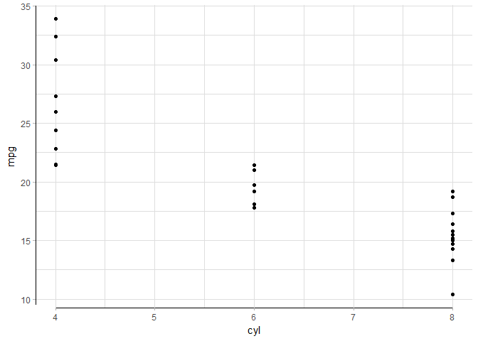

NB: Disable panel.border and enable axis.line in theme, otherwise you will not see an effect!

We could also show that the x-axis is categorical (or ordinal):

r
(p <- ggplot(mtcars, aes(x=as.factor(cyl), y=mpg)) + 
  geompoint(position=positionjitter(width=0.1)) + 
  coordflexcart(bottom=bracketshorisontal(), left=cappedvertical('both')) +
  themelight() + theme(panel.border=elementblank(), axis.line = element_line())
)

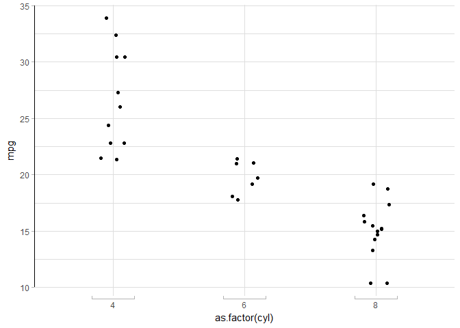
When capping the axis lines, they are never capped further inwards than the ticks! Look up

• coordcappedcart, coordcappedflip
• coordflexcart, coordflexflip, coordflexfixed
• bracketshorisontal, bracketsvertical
• cappedhorisontal, cappedvertical

Having produced such wonderous axes, it is a pity they are not plotted around all panels when using faceting. We have extended both facetgrid and facetwrap to produce axis, ticks, and labels on all panels:

r
p + facetrepwrap(~gear, ncol=2, label=label_both)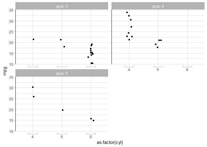

They work just like the normal ones; look up facetrepgrid and facetrepwrap.

geom_pointline

A geom that combines both points and lines. While possible by using both geompoint and geomline, position adjustments are not preserved between the two layers. geompointline and geompointpath combines geompoint with geomline and geom_path, respectively, while preserving position adjustments.

Left: geompoint and geomline as two separate geoms. Right: The two geoms combined into geompointline. Both produced with ggplot(mtcars, aes(wt, mpg, colour=factor(cyl))) + geompoint(col='grey'), where the grey points indicate the true location of the datapoint.

An added visual effect is seen as the lines do not touch the points, leaving a small gap (set by argument distance).

Legends

Reposition the legend onto the plot. Exactly where you want it:

r
dsamp <- diamonds[sample(nrow(diamonds), 1000), ]
d <- ggplot(dsamp, aes(carat, price)) +
  geom_point(aes(colour = clarity))
reposition_legend(d, 'top left')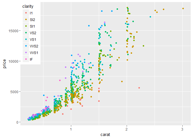

The legend repositioned onto the top left corner of the panel.

Scavenging the Internet, we have found some functions that help work with legends.

Frequently appearing on Stack Overflow, we bring you glegend:

r
library(grid)
legend <- g_legend(d)
grid.newpage()
grid.draw(legend)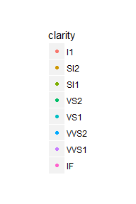

The legend grob, by itself.

Originally brought to you by (Baptiste Auguié)\[\] () and (Shaun Jackman)\[\] (arrangeshared_legend>). We put it in a package.

r
dsamp <- diamonds[sample(nrow(diamonds), 1000), ]
p1 <- qplot(carat, price, data = dsamp, colour = clarity)
p2 <- qplot(cut, price, data = dsamp, colour = clarity)
p3 <- qplot(color, price, data = dsamp, colour = clarity)
p4 <- qplot(depth, price, data = dsamp, colour = clarity)
gridarrangeshared_legend(p1, p2, p3, p4, ncol = 2, nrow = 2)

Four plots that share the same legend.

Extensions to knitr

knitr allows S3 methods for knitprint for specialised printing of objects. We provide lemonprint for data frames, dplyr tables, and summary objects, that can be used to render the output, without mucking up the code source. An added benefit is that we can use RStudio's inline data frame viewer:

Relative file paths made safe

Using knitr for computations that use external binaries and/or write temporary files, setting the root directory for knitr's knitting saves the user from a file mess. E.g.

r
knitr::opts_knit$set(root.dir=TMPDIR)

But we want to keep our file paths relative for the scripts / document to be transferable. We introduce the .dot functions:

r
TMPDIR=tempdir()
.data <- .dot('data')
knitroptsknit$set(root.dir=TMPDIR)

We can then load our data file using the created .data function, even though the chunk is executed from TMPDIR.

r
dat <- read.table(.data('mydata.tab'))