Topics

#a5 #cli-tool #data-science #data-vizualisation #dggs #geohash #geoparquet #geospatial #gis #h3 #maidenhead #map-visualization #parquet #qth #raster #raster-data #rhealpix #s2

Language breakdown

No language data available.

▸ Files click to expand

README

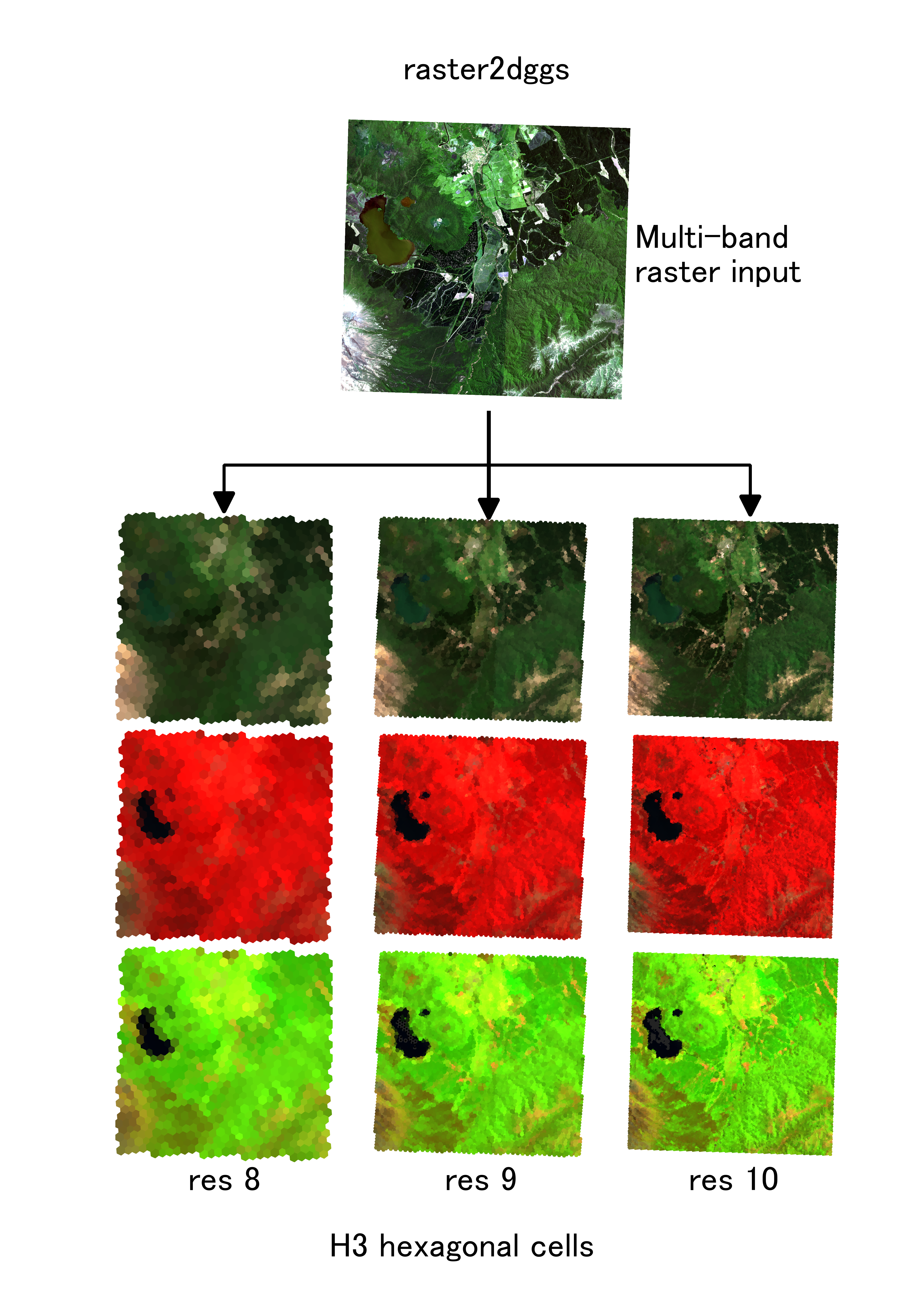
raster2dggs

Python-based CLI tool to index raster files to DGGS in parallel, writing out to Parquet.

This is the raster equivalent of vector2dggs.

Currently this supports the following DGGSs:

H3
rHEALPix
S2
A5
Via DGGAL: ISEA4R, ISEA9R, ISEA3H, ISEA7H, IVEA4R, IVEA9R, IVEA3H, IVEA7H, RTEA4R, RTEA9R, RTEA7H, HEALPix, rHEALPix

And these geocode systems:

Contributions (particularly for additional DGGSs), suggestions, bug reports and strongly worded letters are all welcome.

Example use case for raster2dggs, showing how an input raster can be indexed at different DGGS resolutions, while retaining information in separate, named bands

Installation

This tool makes use of optional extras to allow you to install a limited subset of DGGSs.

If you want all possible:

pip install raster2dggs[all]

If you want only a subset, use the pattern pip install raster2dggs[a5] (for one) or pip install raster2dggs[h3,s2,isea4r] (for multiple).

A bare pip install raster2dggs will not install any DGGS backends.

Usage

raster2dggs --help Usage: raster2dggs [OPTIONS] COMMAND [ARGS]... Options: --version Show the version and exit. --help Show this message and exit.

Commands: a5 Index raster data into the A5 DGGS geohash Index raster data into the Geohash DGGS h3 Index raster data into the H3 DGGS healpix Index raster data into the HEALPix DGGS isea4r Index raster data into the ISEA4R DGGS isea7h Index raster data into the ISEA7H DGGS isea9r Index raster data into the ISEA9R DGGS ivea4r Index raster data into the IVEA4R DGGS ivea7h Index raster data into the IVEA7H DGGS ivea9r Index raster data into the IVEA9R DGGS maidenhead Index raster data into the Maidenhead DGGS rhp Index raster data into the rHEALPix DGGS rtea4r Index raster data into the RTEA4R DGGS rtea7h Index raster data into the RTEA7H DGGS rtea9r Index raster data into the RTEA9R DGGS s2 Index raster data into the S2 DGGS

raster2dggs h3 --help Usage: raster2dggs h3 [OPTIONS] RASTERINPUT OUTPUTDIRECTORY Ingest a raster image and index it to the H3 DGGS. RASTER_INPUT is the path to input raster data; prepend with protocol like s3:// or hdfs:// for remote data. OUTPUT_DIRECTORY should be a directory, not a file, as it will be the write location for an Apache Parquet data store, with partitions equivalent to parent cells of target cells at a fixed offset. However, this can also be remote (use the appropriate prefix, e.g. s3://).

Options: -v, --verbosity LVL Either CRITICAL, ERROR, WARNING, INFO or DEBUG [default: INFO] -r, --resolution [0-15|smaller-than-pixel|larger-than-pixel|min-diff] H3 resolution to index. Accepts an integer in [0, 15] or an auto-detection mode: 'smaller-than-pixel' (first resolution finer than a pixel), 'larger-than-pixel' (last resolution coarser than a pixel), or 'min- diff' (resolution closest to pixel size). [required] -pr, --parent_res INTEGER RANGE H3 parent resolution to index and aggregate to. Defaults to max(0, resolution - 6) [0<=x<=15] -b, --band TEXT Band(s) to include in the output. Can specify multiple, e.g. -b 1 -b 2 -b 4 for bands 1, 2, and 4 (all unspecified bands are ignored). If unused, all bands are included in the output (this is the default behaviour). Bands can be specified as numeric indices (1-based indexing) or string band labels (if present in the input), e.g. -b B02 -b B07 -b B12. -n, --nodata [omit|emit] 'omit' excludes nodata cells from output (default). 'emit' includes them, writing the source raster nodata value (or --nodata-fill if set). Note: non-NaN emitted values participate in cell aggregation (see -a/--agg); if this is undesired, ensure your source nodata is NaN or override with --nodata-fill. [default: omit] --nodata-fill NUMBER Override the value written for nodata cells when --nodata=emit. If omitted, the source raster nodata value is used (NaN if none is defined). Coerced to the output dtype. Note: non-NaN values participate in cell aggregation (see -a/--agg). -c, --compression TEXT Compression method to use for the output Parquet files. Options include 'snappy', 'gzip', 'brotli', 'lz4', 'zstd', etc. Use 'none' for no compression. [default: snappy] -t, --threads INTEGER Number of threads to use when running in parallel. The default is determined dynamically as the total number of available cores, minus one. --point OUTPUT [Mutually exclusive with --overlay and --sample] Assign each pixel to the DGGS cell containing its centre (default). OUTPUT: 'value' (scalar per cell, default), 'list' (sorted list of all contributing pixel values), 'histogram' (value-count struct). --overlay METHOD [Mutually exclusive with --point and --sample] Area-based polygon intersection. METHOD: 'weighted' (area-weighted mean), 'mode' (majority class by overlap area), 'mass-preserve' (area-weighted sum; conserves total — use when pixel value is a total count/mass), 'density-preserve' (integrates density × pixel area; use when pixel value is a per-area rate), 'fractions' (per-class area fractions → struct), 'list' (all overlapping pixel values as a sorted list), 'histogram' (value-count histogram of overlapping pixels). --sample INTERP [Mutually exclusive with --point and --overlay] Sample the raster at each DGGS cell centre. INTERP: 'nn' (nearest- neighbour, default), 'bilinear', 'bicubic', 'lanczos'. -a, --agg AGGFUNC[,AGGFUNC...] Aggregation function(s) applied when multiple raster pixels map to the same DGGS cell (only relevant for --point). Options: count, mean, sum, prod, std, var, min, max, median, mode, majority, nunique, range. Comma-separate multiple names (e.g. min,max) to produce a struct column per band. [default: mean] -vct, --valid-coverage-threshold FLOAT RANGE Minimum fraction of each DGGS cell's overlapping raster area that must contain valid (non-nodata) pixels for the cell to receive a value. Applied per band. 0.0 (default) keeps all cells with any valid data. Only meaningful for --overlay; ignored for --overlay mass-preserve (partial sums are correct values — filtering them would break mass conservation). [default: 0.0; 0.0<=x<=1.0] -d, --decimals INTEGER|none Decimal places to round output values. 0 = integer; negative values round to tens (-1), hundreds (-2), etc. Use 'none' to disable rounding. [default: 1] -o, --overwrite -co, --compact Compact the cells up to the parent resolution. Compaction is only applied where all sibling cells share identical values in every output column. -g, --geo [point|polygon|none] Write output as a GeoParquet (v1.1.0) with either point or polygon geometry. [default: none] --tempdir PATH Temporary data is created during the execution of this program. This parameter allows you to control where this data will be written. --version Show the version and exit. --help Show this message and exit.

Sampling strategies

Three mutually exclusive modes control how pixel values are mapped to DGGS cells:

--point (default) — index each pixel centre to a DGGS cell
--overlay METHOD — compute area-weighted intersections between pixels and DGGS cells
--sample — sample the raster at each DGGS cell centre

Point sampling (default) — `--point`

Each raster pixel centre is indexed to its containing DGGS cell. When multiple pixels fall in the same cell, -a/--agg determines how they are combined (default: mean). Produces sparse output (gaps) when the DGGS resolution is finer than the raster.

Output modes (pass as --point OUTPUT):

(no arg / --point value) — scalar per cell per band; use --agg min,max etc. for multi-agg struct output
--point list — sorted list of all contributing pixel values: list<T> per band. --agg is ignored.
--point histogram — value-count histogram: struct<values: list<T>, counts: list<int64>> per band. --agg is ignored.

# Default: mean of all contributing pixels raster2dggs h3 input.tif output/ -r 9
Min and max in a single pass
raster2dggs h3 input.tif output/ -r 9 --agg min,max
Sorted list of all pixel values per cell
raster2dggs h3 input.tif output/ -r 7 --point list -d 2
Histogram of pixel values per cell
raster2dggs h3 input.tif output/ -r 7 --point histogram -d 0

Overlay (area-based) — `--overlay METHOD`

Uses exactextract to compute exact pixel–cell intersection areas. METHOD is required:

| --overlay METHOD | Output schema | Use for | |---|---|---| | weighted | Scalar T per band | Intensive quantities: temperature, elevation, concentration, fraction cover — value per unit area, averaged across the cell | | mode | Scalar T per band | Categorical rasters: land cover, soil type, zone IDs, masks | | mass-preserve | Scalar T per band | Extensive totals: population count, emissions — pixel value is already a total; sum is conserved | | density-preserve | Scalar T per band | Density rasters (W/m², kg/km²) — integrates density × pixel area to give the cell total; geographic CRS uses geodesic pixel areas | | fractions | struct<classes: list<int64>, fractions: list<float64>> per band | Class area fractions within each DGGS cell | | list | list<T> per band | All overlapping pixel values as a sorted list (collect mode) | | histogram | struct<values: list<T>, counts: list<int64>> per band | Histogram of overlapping pixel values |

# Area-weighted mean (intensive quantities)
raster2dggs h3 input.tif output/ -r 8 --overlay weighted
Majority-class (categorical rasters)
raster2dggs h3 landcover.tif output/ -r 8 --overlay mode
Mass-conserving sum (population counts)
raster2dggs h3 popcount.tif output/ -r 8 --overlay mass-preserve
Density integration (W/m² → total W per DGGS cell)
raster2dggs h3 power_density.tif output/ -r 8 --overlay density-preserve
Per-class area fractions
raster2dggs h3 landcover.tif output/ -r 8 --overlay fractions
Collect all overlapping pixel values as a list
raster2dggs h3 input.tif output/ -r 8 --overlay list
Histogram of all overlapping pixel values
raster2dggs h3 input.tif output/ -r 8 --overlay histogram

Performance note

--overlay uses exactextract to compute pixel–cell area intersections. For each raster window, exactextract reads only the raster blocks needed to cover that window's DGGS cells. If the raster fits in memory, increasing GDAL's block cache allows blocks read for early windows to remain cached for later ones, reducing redundant I/O:

GDAL_CACHEMAX=512 raster2dggs h3 input.tif output/ -r 8 --overlay weighted

The value is in megabytes. The default is 64 MB. For large rasters or high DGGS resolutions where each window covers many cells, a larger cache can significantly reduce processing time.

Valid-data coverage threshold (`-vct` / `--valid-coverage-threshold`)

By default (-vct 0.0) any cell with at least one valid pixel in its overlap area receives a value. Use --valid-coverage-threshold to require a minimum fraction of the cell's raster-overlapping area to have valid (non-nodata) data:

# Discard cells where fewer than 50% of overlapping pixels are valid
raster2dggs h3 input.tif output/ -r 8 --overlay mode -vct 0.5

The threshold is applied per band: a cell may receive a valid value for one band and be nulled for another if that band has sparser nodata. Nulled values are then handled by --nodata — the default omit drops rows where any band is null; emit keeps them as NaN (or --nodata-fill if set).

This option has no effect for --overlay mass-preserve. Partial sums produced by mass-preserve are correct values representing the fraction of mass within the cell–raster intersection; filtering them out would break the mass-conservation guarantee. --overlay density-preserve respects the threshold normally — a cell with insufficient valid coverage will be nulled.

Windowed resampling — `--sample`

For each DGGS cell, samples the raster at the cell centre using windowed I/O. Pass the resampling kernel as --sample INTERP (default: nn):

| INTERP | Description | |---|---| | nn (default) | Nearest-neighbour — suitable for categorical rasters | | bilinear | Bilinear (2×2 stencil) — smooth continuous fields | | bicubic | Bicubic/Keys (4×4 stencil) — higher-quality smooth fields | | lanczos | Lanczos-3 (6×6 stencil) — highest quality, slowest |

# NN sample (default — works for both continuous and categorical)
raster2dggs h3 input.tif output/ -r 9 --sample
Bilinear sample for a smooth continuous field (DEM, temperature)
raster2dggs h3 dem.tif output/ -r 9 --sample bilinear
NN sample for a categorical raster (landcover)
raster2dggs h3 landcover.tif output/ -r 9 --sample -d 0

--agg is ignored for --sample. Supports --compact.

Visualising output

Output is in the Apache Parquet format, hive partitioned with the parent resolution as partition key. The example below is with -pr 3 with the H3 DGGS.

tree /home/user/example.pq

/home/user/example.pq ├── h3_03=83bb09fffffffff │ └── part.0.parquet └── h3_03=83bb0dfffffffff └── part.0.parquet

Output can also be written to GeoParquet (v1.1.0) by including the -g/--geo parameter, which accepts:

polygon for cells represented as boundary polygons
point for cells represented as centre points
none for standard Parquet output (not GeoParquet) ← this is the default if -g/--geo is not used

GeoParquet output is useful if you want to use the spatial representations of the DGGS cells in traditional spatial analysis, or if you merely want to visualise the output.

Below are some ways to read and visualise it.

DuckDB

$ duckdb
DuckDB v1.4.1 (Andium) b390a7c376
Enter ".help" for usage hints.
Connected to a transient in-memory database.
Use ".open FILENAME" to reopen on a persistent database.
D INSTALL spatial;
D LOAD spatial;
D SELECT * FROM readparquet('seisland.pq') LIMIT 7;
┌────────┬────────┬────────┬────────────────────────────────────────────────────────────────────────────────┬─────────────┬─────────┐
│ band1 │ band2 │ band3 │                                    geometry                                    │    s219    │  s2_08  │
│ float  │ float  │ float  │                                    geometry                                    │   varchar   │ varchar │
├────────┼────────┼────────┼────────────────────────────────────────────────────────────────────────────────┼─────────────┼─────────┤
│    0.0 │    0.0 │    0.0 │ POLYGON ((-176.17946725380486 -44.33542073938414, -176.17946725380486 -44.33…  │ 72b47e01e24 │ 72b47   │
│    0.0 │    0.0 │    0.0 │ POLYGON ((-176.18439390505398 -44.33543749229784, -176.18439390505398 -44.33…  │ 72b47e02a14 │ 72b47   │
│    0.0 │    0.1 │    0.1 │ POLYGON ((-176.18550630891403 -44.33547457195554, -176.18550630891403 -44.33…  │ 72b47e1d54c │ 72b47   │
│    0.0 │    0.0 │    0.0 │ POLYGON ((-176.17819578278952 -44.33537828938332, -176.17819578278952 -44.33…  │ 72b47e01d64 │ 72b47   │
│    0.1 │    0.1 │    0.3 │ POLYGON ((-176.18344039674218 -44.335553297533835, -176.18344039674218 -44.3…  │ 72b47e0282c │ 72b47   │
│    0.0 │    0.0 │    0.0 │ POLYGON ((-176.17899045588274 -44.335404822417665, -176.17899045588274 -44.3…  │ 72b47e01dfc │ 72b47   │
│    0.1 │    0.1 │    0.3 │ POLYGON ((-176.1832814769592 -44.33554799806149, -176.1832814769592 -44.3356…  │ 72b47e02824 │ 72b47   │
└────────┴────────┴────────┴────────────────────────────────────────────────────────────────────────────────┴─────────────┴─────────┘

Output value columns may also be arrays (double[] or int64[]) or structs, not just scalar values, depending on the options you pass to the tool (e.g. --agg min,max (multiple aggregations) or --point list/--point histogram) and the relative size of the DGGS cells and raster cells.

In the case of struct outputs, it should be noted that there's no real consequence of using a struct (i.e. band1.min, band1.max) over a series of flat columns (i.e. band1min, band1max), since Parquet uses Dremel shredding for nested types: a struct(min double, max double) column is physically stored as two separate column chunks (band1.min, band1.max) with definition/repetition level metadata. So the on-disk layout is identical to flat columns. Consequences:

Compression: identical. The min values are stored contiguously together, max values together, same as flat columns. Encoding schemes (dictionary, RLE, delta) apply the same way.
Column pruning / projection pushdown: also identical for modern readers. DuckDB's SELECT band1.min FROM ... reads only the min sub-column chunk, same as SELECT band1_min FROM ... would with flat columns.
Definition level overhead: structs add a small amount of metadata to encode nullability at each nesting level. For non-nullable structs with non-nullable fields this is negligible: a few bytes per row group.

Examples:

--point list -d 1:

D SELECT band1 FROM readparquet('./tests/data/output/larger-than-pixel/tempmeanwgs84-poly.geoparquet') LIMIT 7;
┌────────────────────────────────────────────┐
│                   band_1                   │
│                  double[]                  │
├────────────────────────────────────────────┤
│ [15.9, 15.9, 16.1, 16.1, 16.3, 16.3]       │
│ [16.0, 16.0, 16.0, 16.1, 16.1, 16.2, 16.2] │
│ [16.4, 16.6, 16.7, 16.7, 17.0, 17.1]       │
│ [18.0, 18.2, 18.3, 18.4, 18.5]             │
│ [16.4, 16.5, 16.5, 16.6, 16.8, 16.8]       │
│ [17.4, 17.6, 17.7, 17.9, 18.0, 18.2]       │
│ [16.1, 16.2, 16.2, 16.3, 16.4, 16.5]       │
└────────────────────────────────────────────┘

--point histogram -d 0:

D SELECT band1 FROM readparquet('./tests/data/output/larger-than-pixel/tempmeanwgs84-poly.geoparquet') LIMIT 7;
┌────────────────────────────────────────────┐
│                   band_1                   │
│ struct("values" bigint[], counts bigint[]) │
├────────────────────────────────────────────┤
│ {'values': [16], 'counts': [6]}            │
│ {'values': [16], 'counts': [7]}            │
│ {'values': [16, 17], 'counts': [1, 5]}     │
│ {'values': [18], 'counts': [5]}            │
│ {'values': [16, 17], 'counts': [2, 4]}     │
│ {'values': [17, 18], 'counts': [1, 5]}     │
│ {'values': [16, 17], 'counts': [5, 1]}     │
└────────────────────────────────────────────┘

--agg min,max,majority,mode -d 0:

D SELECT band1 FROM readparquet('./tests/data/output/larger-than-pixel/tempmeanwgs84-poly.geoparquet') LIMIT 7;
┌────────────────────────────────────────────────────────────────┐
│                             band_1                             │
│ struct(min bigint, max bigint, majority bigint, "mode" bigint) │
├────────────────────────────────────────────────────────────────┤
│ {'min': 16, 'max': 16, 'majority': 16, 'mode': 16}             │
│ {'min': 16, 'max': 16, 'majority': 16, 'mode': 16}             │
│ {'min': 16, 'max': 17, 'majority': 17, 'mode': 17}             │
│ {'min': 18, 'max': 18, 'majority': 18, 'mode': 18}             │
│ {'min': 16, 'max': 17, 'majority': 17, 'mode': 17}             │
│ {'min': -9999, 'max': 18, 'majority': 18, 'mode': 18}          │
│ {'min': 16, 'max': 17, 'majority': 16, 'mode': 16}             │
└────────────────────────────────────────────────────────────────┘

GDAL

ogrinfo -so -al ./se_island.pq
INFO: Open of se_island.pq&#39;
      using driver Parquet' successful.
Layer name: se_island Geometry: Polygon Feature Count: 18390 Extent: (-176.185824, -44.356933) - (-176.159915, -44.335364) Layer SRS WKT: GEOGCRS["WGS 84",     ENSEMBLE["World Geodetic System 1984 ensemble",         MEMBER["World Geodetic System 1984 (Transit)"],         MEMBER["World Geodetic System 1984 (G730)"],         MEMBER["World Geodetic System 1984 (G873)"],         MEMBER["World Geodetic System 1984 (G1150)"],         MEMBER["World Geodetic System 1984 (G1674)"],         MEMBER["World Geodetic System 1984 (G1762)"],         MEMBER["World Geodetic System 1984 (G2139)"],         MEMBER["World Geodetic System 1984 (G2296)"],         ELLIPSOID["WGS 84",6378137,298.257223563,             LENGTHUNIT["metre",1]],         ENSEMBLEACCURACY[2.0]],     PRIMEM["Greenwich",0,         ANGLEUNIT["degree",0.0174532925199433]],     CS[ellipsoidal,2],         AXIS["geodetic latitude (Lat)",north,             ORDER[1],             ANGLEUNIT["degree",0.0174532925199433]],         AXIS["geodetic longitude (Lon)",east,             ORDER[2],             ANGLEUNIT["degree",0.0174532925199433]],     USAGE[         SCOPE["Horizontal component of 3D system."],         AREA["World."],         BBOX[-90,-180,90,180]],     ID["EPSG",4326]] Data axis to CRS axis mapping: 2,1 Geometry Column = geometry band_1: Real(Float32) (0.0) band_2: Real(Float32) (0.0) band_3: Real(Float32) (0.0) s2_19: String (0.0) s2_08: String (0.0)

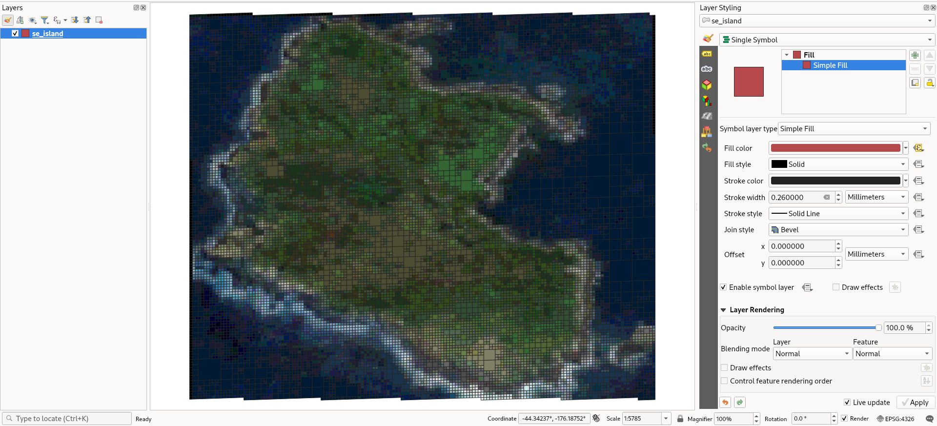
QGIS

qgis sample.pq

With some styling applied:

Example output shown in QGIS

Installation (detailed)

PyPi:

pip install raster2dggs[all]

Conda environment:

name: raster2dggs
channels:
  - conda-forge
channel_priority: strict
dependencies:
  - python>=3.11,<3.12
  - pip=23.1.*
  - gdal>=3.8.5
  - pyproj=3.6.*
  - pip:
    - raster2dggs[all]>=0.9.0

For development

In brief, to get started:

Install Poetry
Install GDAL

- If you're on Windows, pip install gdal may be necessary before running the subsequent commands. - On Linux, install GDAL 3.6+ according to your platform-specific instructions, including development headers, i.e. libgdal-dev.

Create the virtual environment with poetry install. This will install necessary dependencies.
Subsequently, the virtual environment can be re-activated with poetry env activate.

If you run poetry install -E all --with dev, the CLI tool will be aliased so you can simply use raster2dggs rather than poetry run raster2dggs, which is the alternative if you do not poetry install -E all --with dev.

For partial backend support you can consider poetry install --with dev -E h3 -E a5 etc. To check what is installed: poetry show --tree.

Code formatting

Please run black . before committing.

Tests

Tests are included. To run them, set up a poetry environment, then run from the project root:

pytest -v --durations=10 --tb=short

-v — one line per test with pass/fail status
--durations=10 — reports the 10 slowest tests at the end
--tb=short — compact tracebacks on failure
Add -x to stop on the first failure when debugging

To run a subset of tests:

pytest -k h3                        # all tests whose ID contains "h3"
pytest -k "h3 or rhp"
pytest -k "sample and rhp"
pytest tests/classes/testsamplenn.py          # sample transfer smoke tests
pytest "tests/classes/testcliintegration.py::TestAllDGGS::test_command[h3-polygon-co]"  # exact parametrised case

Test data are included at tests/data/.

Generating synthetic sample rasters

make_samples.py generates a small suite of synthetic GeoTIFF rasters for experimentation. It only requires numpy and rasterio (plus optional scipy for better smoothing):

python makesamples.py --outdir samplerasters --seed 42

This writes six rasters to sample_rasters/:

| File | Semantics | Nodata pattern | CRS | |---|---|---|---| | landcoverutm33.tif | piecewiseconstant — 6 landcover classes | Scattered holes + missing stripe | UTM 33N | | fractreecoverutm33.tif | fraction_cover — tree cover 0–1 | Coastline-shaped mask | UTM 33N | | popcountwebmerc.tif | counttotal — heavy-tailed counts | Rotated rectangle polygon | Web Mercator | | tempmeanwgs84.tif | cell_average — continuous temperature | Edge band + scattered pixels | WGS84 | | zoneidslaea.tif | piecewise_constant — Voronoi zone IDs | Islands + sliver patches | Europe LAEA | | multibandperbandnodatawgs84.tif | 4-band float32 | Nodata at different pixels per band | WGS84 | | swathwgs84.tif | pointcenter_strict — 3-band simulated swath | ~85% nodata outside diagonal strip; bbox ~6× larger than data footprint | WGS84 (diagonal NE–SW strip within 120–160°E, 20–60°N; swath widens northward via geodesic cross-track mask) | | swathpolarstereo.tif | pointcenterstrict — 3-band simulated swath | Thin nodata margins at swath edges | Arctic polar stereographic (custom CRS); rectangular grid in CRS appears as a curved arc across ~38–80°N, ~148–172°E in WGS84 — exercises CRS reprojection code path | | swathushape.tif | pointcenterstrict — 1-band continuous | No nodata | EPSG:3031 (Antarctic polar stereo); all four corners at ~21–26°N in WGS84, but the bottom edge centre is at ~11°N — a naive corner-only bbox misses ~10° of southward extent |

The multi-band raster is specifically designed to exercise per-band nodata handling: a pixel that is nodata in one band can be valid in another.

Experimenting

Two sample files have been uploaded to an S3 bucket with s3:GetObject public permission.

s3://raster2dggs-test-data/Sen2_Test.tif (sample Sentinel 2 imagery, 10 bands, rectangular, Int16, LZW compression, ~10x10m pixels, 68.6 MB)
s3://raster2dggs-test-data/TestDEM.tif (sample LiDAR-derived DEM, 1 band, irregular shape with null data, Float32, uncompressed, 10x10m pixels, 183.5 MB)

You may use these for experimentation. However you can also use local files too, which will be faster. A good, small (5 MB) sample image is available here.

A small test file is also available at tests/data/se-island.tif.

You can also generate a suite of synthetic rasters locally using make_samples.py — see Generating synthetic sample rasters above.

Example commands

Index to H3 at resolution 11, integer output:

raster2dggs h3 --resolution 11 -d 0 s3://raster2dggs-test-data/Sen2Test.tif ./tests/data/output/11/Sen2Test

Same raster to rHEALPix:

raster2dggs rhp --resolution 11 -d 0 s3://raster2dggs-test-data/Sen2Test.tif ./tests/data/output/11/Sen2Test_rhp

DEM indexed to H3, median aggregation, GeoParquet polygon output:

raster2dggs h3 --resolution 13 --compression zstd --agg median -d 1 --geo polygon s3://raster2dggs-test-data/TestDEM.tif ./tests/data/output/13/TestDEM

Auto-select resolution (first H3 resolution finer than the raster pixel size):

raster2dggs h3 --resolution smaller-than-pixel input.tif ./output

Multi-aggregation struct output — min, max, and mean per band in one pass:

raster2dggs h3 --resolution 9 --agg min,max,mean -d 1 input.tif ./output

Collect all contributing pixel values per cell as a sorted list:

raster2dggs h3 --resolution 7 --point list -d 2 input.tif ./output

Histogram of contributing pixel values per cell:

raster2dggs h3 --resolution 7 --point histogram -d 0 input.tif ./output

Nearest-neighbour sampling for a continuous field (e.g. DEM, temperature grid):

raster2dggs h3 --resolution 9 --sample input.tif ./output

Bilinear sampling for a continuous field:

raster2dggs h3 --resolution 9 --sample bilinear input.tif ./output

Nearest-neighbour sampling for a categorical raster (e.g. landcover):

raster2dggs h3 --resolution 9 --sample -d 0 landcover.tif ./output

Area-weighted mean for a continuous raster:

raster2dggs h3 --resolution 8 --overlay weighted input.tif ./output

Majority-class for a categorical raster:

raster2dggs h3 --resolution 8 --overlay mode landcover.tif ./output

Mass-conserving sum for population counts:

raster2dggs h3 --resolution 8 --overlay mass-preserve popcount.tif ./output

Emit nodata cells rather than omitting them, replacing the nodata value with −1:

raster2dggs h3 --resolution 9 --nodata emit --nodata-fill -1 input.tif ./output

Citation

Citation metadata is maintained in CITATION.cff. GitHub renders this as a "Cite this repository" button on the repository page (top-right of the About panel), which provides ready-to-copy BibTeX and APA formats.