ML Cheatsheet

Assuming we have the dataset in a loadable format (e.g., csv), here are the steps we follow to complete a machine learning project.

• Exploratory data analysis
• Preprocessing
• Feature engineering
• Machine learning

A couple of notes before we go on.

First of all, machine learning is a highly iterative field. This would entail a loop cycle of the above steps, where each cycle is based on the feedback from the previous cycle, with the goal of improving the model performance. One example is that we need refit models when we engineered new features, and test to see if these features are predicative.

Second, while in Kaggle competitions one can create a monster ensemble of models, in production system often times such ensembles are not useful. They are high maintenance, hard to interpret, and too complex to deploy. This is why in practice it's often simpler model plus huge amount of data that wins.

Third, while some code snippets are reusable, each dataset has its own uniqueness. Dataset-specific efforts are needed to build better models.

Bearing these points in mind, let's get our hands dirty.

Exploratory data analysis

Exploratory data analysis (EDA) is an approach to analyze data sets to summarize their main characteristics, often with plots. The goal of EDA is to get a deeper understanding of the dataset, and to preprocess data and engineer features more effectively. Here are some generic code snippets that can be applied to any structured dataset

import libraries

import os import fnmatch import glob import numpy as np import pandas as pd import matplotlib.pyplot as plt import seaborn as sns

data I/O

df = pd.readcsv(filepath) # read in csv file as a DataFrame df.tocsv(filepath, index=False) # save a DataFrame as csv file

read all csv under a folder and concatenate them into a big dataframe
path = r'path'
flat
all_files = glob.glob(os.path.join(path, "*.csv"))
or recursively
all_files = [os.path.join(root, filename)
             for root, dirnames, filenames in os.walk(path)
             for filename in fnmatch.filter(filenames, '*.csv')]
             
df = pd.concat((pd.readcsv(f) for f in allfiles))

data I/O zipped

import pandas as pd
import zipfile
zf_path = 'file.zip' zf = zipfile.ZipFile(zf_path) # zipfile.ZipFile object all_files = zf.namelist() # list all zipped files allfiles = [f for f in allfiles if f.endswith('.csv')] # e.g., get only csv df = pd.concat((pd.readcsv(zf.open(f)) for f in allfiles)) # concat all zipped csv into one dataframe

To a table in sqlite3 DB (then you can use DB Browser for SQLite to view and query the table)

import sqlite3
import pandas as pd
df = pd.readcsv(csvfile) # read csv file sqlitefile = 'mydb.sqlite3' conn = sqlite3.connect(sqlite_file) # establish a sqlite3 connection
if db file exists append the csv
df.tosql(tablename, conn, ifexists='append', index=False)

data summary

df.head() # return the first 5 rows df.describe() # summary statistics, excluding NaN values df.info(verbose=True, null_counts=True) # concise summary of the table df.shape # shape of dataset df.skew() # skewness for numeric columns df.kurt() # unbiased kurtosis for numeric columns df.getdtypecounts() # counts of dtypes

display missing value proportion for each col

for c in df.columns:   num_na = df[c].isnull().sum()   if num_na > 0:     print round(num_na / float(len(df)), 3), '|', c

pairwise correlation of columns

df.corr()

plotting

plot heatmap of correlation matrix (of all numeric columns)

cm = np.corrcoef(df.T) sns.heatmap(cm, annot=True, yticklabels=df.columns, xticklabels=df.columns)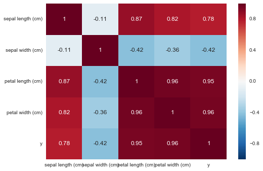

plot univariate distributions

# single column sns.distplot(df['col1'].dropna())

all numeric columns
for c in df.columns:
  if df[c].dtype in ['int64', 'float64']:
    sns.distplot(df[c].dropna(), kde=False)
    plt.show()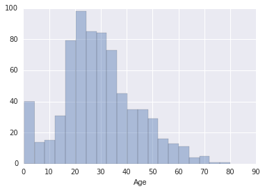

plot kernel density estimaton (KED)

# all continuous variables for c in df.columns:   if df[c].dtype in ['float64']:     sns.kdeplot(df[c].dropna(), shade=True)     plt.show()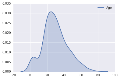

plot pairwise relationships

sns.pairplot(df.dropna())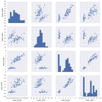

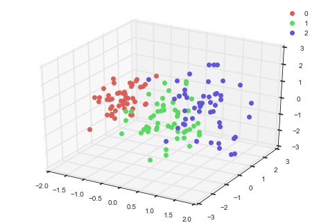
**hypertools is a python toolbox for visualizing and manipulating high-dimensional data. This is desirable for the EDA phase.**

visually explore relationship between features and target (in 3D space)

import hypertools as hyp import seaborn as sns from sklearn import datasets

iris = datasets.load_iris() X = iris.data y = iris.target hyp.plot(X,'o', group=y, legend=list(set(y)), normalize='across')

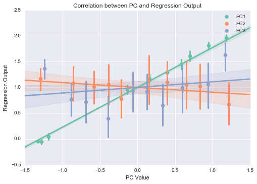
linear regression analysis using each PC

from sklearn import linear_model sns.set(style="darkgrid") sns.set_palette(palette='Set2')

data = pd.DataFrame(data=X, columns=iris.feature_names) reduced_data = hyp.reduce(hyp.tools.df2mat(data), ndims=3)
linreg = linear_model.LinearRegression() linreg.fit(reduced_data, y)
sns.regplot(x=reduceddata[:,0],y=linreg.predict(reduceddata), label='PC1',x_bins=10) sns.regplot(x=reduceddata[:,1],y=linreg.predict(reduceddata), label='PC2',x_bins=10) sns.regplot(x=reduceddata[:,2],y=linreg.predict(reduceddata), label='PC3',x_bins=10)
plt.title('Correlation between PC and Regression Output') plt.xlabel('PC Value') plt.ylabel('Regression Output') plt.legend() plt.show()

break down by labels

sns.set(style="darkgrid") sns.swarmplot(y,reduced_data[:,0],order=[0, 1, 2]) plt.title('Correlation between PC1 and target') plt.xlabel('Target') plt.ylabel('PC1 Value') plt.show()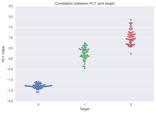

For more use cases of hypertools, check notebooks and examples

Preprocessing

drop columns

df.drop([col1, col2, ...], axis=1, inplace=True) # in place new_df = df.drop([col1, col2, ...], axis=1) # create new df (overhead created)

handle missing values

# fill with mode, mean, or median dfmode, dfmean, df_median = df.mode().iloc[0], df.mean(), df.median()

dffillmode = df.fillna(df_mode) dffillmean = df.fillna(df_mean) dffillmedian = df.fillna(df_median)
drop col with any missing values
dfdropna_col = df.dropna(axis=1)

encode categorical features

from sklearn.preprocessing import LabelEncoder

df_col = df.columns colnonnum = [c for c in df_col if df[c].dtype == 'object'] for c in colnonnum:   df[c] = LabelEncoder().fit_transform(df[c])

join two tables/dataframes

df1.join(df2, on=col)

handle outliners (outliers can either be clipped, or removed. WARNING: outliers are not always meant to be removed)

In the following example we assume df is all numeric, and has no missing values

clipping

# clip outliers to 3 standard deviation lower = df.mean() - df.std()*3 upper = df.mean() + df.std()*3 clipped_df = df.clip(lower, upper, axis=1)

removal

# remove rows that have outliers in at least one column new_df = df[(np.abs(stats.zscore(df)) < 3).all(axis=1)]

filter

# filter by one value new_df = df[df.col==val]

filter by multiple values
newdf = df[df.col.isin(vallist)]

Feature engineering

Transformation

one-hot encode categorical features; not necessary for tree-based algorithms

# for a couple of columns onehotdf = pd.get_dummies(df[[col1, col2, ...]])

for the whole dataframe
newdf = pd.getdummies(df)

normalize numeric features (to range [0, 1])

from sklearn.preprocessing import MinMaxScaler

scaler = MinMaxScaler() normalizeddf = MinMaxScaler().fittransform(df)

log transformation: for columns with highly skewed distribution, we can apply the log transformation

from scipy.special import log1p transformed_col = df[col].apply(log1p)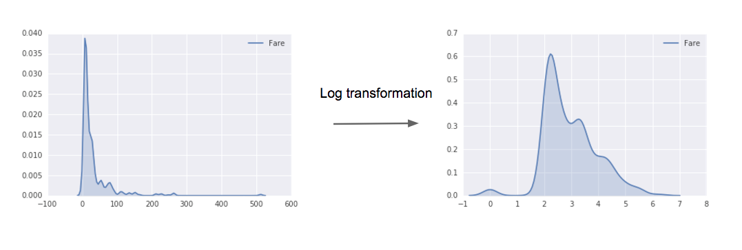

Creation

Feature creation is both domain and engineering efforts. With the help from domain experts, we can craft more predicative features, but here are some generic feature creation methods worth trying on any structured dataset

add feature: number of missing values

df['num_null'] = df.isnull().sum(axis=1)

add feature: number of zeros

df['num_zero'] = (df == 0).sum(axis=1)

add feature: binary value for each feature indicating whether a data point is null

for c in df:   if pd.isnull(df[c]).any():     df[c+'-ISNULL'] = pd.isnull(df[c])

add feature interactions

from sklearn.preprocessing import PolynomialFeatures

e.g., 2nd order interaction
poly = PolynomialFeatures(degree=2)
numpy array of transformed df
arr = poly.fit_transform(df)
all features names
targetfeaturenames = ['x'.join(
    ['{}^{}'.format(pair[0], pair[1]) for pair in tuple if pair[1] != 0])
    for tuple in [zip(Xtrain.columns, p) for p in poly.powers]]
newdf = pd.DataFrame(arr, columns=targetfeature_names)

Selection

There are various ways to select features, and an effective one is recursive feature elimination (RFE).

select feature using RFE

from sklearn.feature_selection import RFE
model = ... # a sklean's classifier that has either 'coef' or 'featureimportances_' attribute num_feautre = 10 # say we want the top 10 features
selector = RFE(model, num_feature, step=1) selector.fit(Xtrain, ytrain) # select features featureselected = list(Xtrain.columns[selector.support_])
model.fit(Xtrain[featureselected], y_train) # re-train a model using only selected features

For more feature engineering methods please refer to this blogpost.

Machine learning

Cross validation (CV) strategy

Theories first (some adopted from Andrew Ng). In machine learning we usually have the following subsets of data:

• training set is used to run the learning algorithm on
• dev set (or hold out cross validation set) is used to tune parameters,

select features, and make other decisions regarding the learning algorithm

• test set is used to evaluate the performance of the algorithms,

but NOT to make any decisions about what algorithms or parameters to use

Ideally, those 3 sets should come from the same distribution, and reflect what data you expect to get in the future and want to do well on.

If we have real-world application from which we continuously collect new data, then we can train on historical data, and split the in-coming data into dev and test sets. This is out of the scope of this cheatsheet. The following exmample assume we have a csv file and we want to train a best model on this snapshot.

How should we split the the three sets? Here is one good CV strategy

• training set the larger the merrier of course :)
• dev set should be large enough to detect differences between algorithms

(e.g., classifier A has 90% accuracy and classifier B has 90.1% then a dev set of 100 examples would not be able to detect this 0.1% difference. Something around the 1,000 to 10,000 will do)

• test set should be large enough to give high confidence in the overall

performance of the system (do not naively use 30% of the data)

Sometimes we can be pretty data strapped (e.g., 1000 data points), and a compromising strategy is 70%/15%/15% for train/dev/test sets, as follows:

from sklearn.modelselection import traintest_split
set seed for reproducibility & comparability
seed = 2017
Xtrain, Xother, ytrain, yother = traintestsplit(   X, y, testsize=0.3, randomstate=seed) Xdev, Xtest, ydev, ytest = traintestsplit(   Xrest, yrest, testsize=0.5, randomstate=seed)

As noted we need to seed the split.

If we have class imbalance issue, we should split the data in a stratified way (using the label array):

Xtrain, Xother, ytrain, yother = traintestsplit(
  X, y, testsize=0.3, randomstate=seed, stratify=y)

Model training

If we've got so far, training is actually the easier part. We just initialize a classifier and train it!

from sklearn.linear_model import LogisticRegression
clf = LogisticRegression() clf.fit(Xtrain, Xtest)

Evaluation

Having a single-number evaluation metric allows us to sort all models according to their performance on this metric and quickly decide what is working best. In production system if we have multiple (N) evaluation metrics, we can set N-1 of the criteria as 'satisficing' metrics, i.e., we simply require that they meet a certain value, then define the final one as the 'optimizing' metric which we directly optimize.

Here is an example of evaluating a model with Area Under the Curve (AUC)

from sklearn.metrics import rocaucscore
ypred = clf.predict(Xtest) print 'ROC score: {}'.format(rocaucscore(ytest, ypred))

Hyperparameter tuning

example of nested cross-validation

import numpy as np
from sklearn.grid_search import GridSearchCV
from sklearn.crossvalidation import crossval_score
from sklearn.ensemble import RandomForestClassifier
X_train = ... # your training features y_train = ... # your training labels
gs = GridSearchCV(   estimator = RandomForestClassifier(random_state=0),   param_grid = {     'n_estimators': [100, 200, 400, 600, 800],      # other params to tune      }   scoring = 'roc_auc',   cv = 5 )
scores = crossvalscore(   gs,   X_train,   y_train,   scoring = 'roc_auc',   cv = 2 )
print 'CV roc_auc: %.3f +/- %.3f' % (np.mean(scores), np.std(scores))

Ensemble

Please refer to the last section of this blogpost.