hrbrmstr/hrbrthemes — 1.4k Stars

Topics

#data-visualization #datavisualization #ggplot-extension #ggplot2 #ggplot2-scales #ggplot2-themes #r #rstats #visualization

Language breakdown

No language data available.

▸ Files click to expand

README

downloads

hrbrthemes

Additional Themes and Theme Components for ‘ggplot2’

This is a very focused package that provides typography-centric themes and theme components for ggplot2.

The core theme: theme_ipsum (“ipsum” is Latin for “precise”) uses Arial Narrow which should be installed on practically any modern system, so it’s “free”-ish. This font is condensed, has solid default kerning pairs and geometric numbers. That’s what I consider the “font trifecta” must-have for charts. An additional quality for fonts for charts is that they have a diversity of weights. Arial Narrow (the one on most systems, anyway) does not have said diversity but this quality is not (IMO) a “must have”.

The following functions are implemented/objects are exported:

Themes:

theme_ipsum: Arial Narrow
themeipsumgs: Goldman Sans Condensed
themeipsumes: Econ Sans Condensed
themeipsumrc: Roboto Condensed
themeipsumps: IBM Plex Sans font
themeipsumpub: Public Sans
themeipsumtw: Titilium Web
thememodernrc: Roboto Condensed dark theme
themeftrc: Dark theme based on FT’s dark theme (Roboto Condensed)

Scales (that align with various themes):

scalecoloripsum: Discrete color & fill scales based on the ipsum

palette

scalecolouripsum: Discrete color & fill scales based on the ipsum

palette

scalefillipsum: Discrete color & fill scales based on the ipsum

palette

scalecolorft: Discrete color & fill scales based on the FT palette
scalecolourft: Discrete color & fill scales based on the FT

palette

scalefillft: Discrete color & fill scales based on the FT palette
scalexcomma: X & Y scales with opinionated presets for percent &

comma label formats

scalexpercent: X & Y scales with opinionated presets for percent &

comma label formats

scaleycomma: X & Y scales with opinionated presets for percent &

comma label formats

scaleypercent: X & Y scales with opinionated presets for percent &

comma label formats

Palettes/Named Colors:

ipsum_pal: A muted, qualitative color palette
ft_cols: FT color palette
ft_pal: A bright qualitative color palette
fttextcol: FT color palette
bit12: A vector of 12 vibrant colors for categorical data
bit12_extended: List of 12 color palettes with 9 shades each for

continuous interpolation

Fonts:

font_an: Arial Narrow font name R variable aliases
font_es: Econ Sans font name R variable aliases
fontesbold: Econ Sans font name R variable aliases
fonteslight: Econ Sans font name R variable aliases
font_rc: Roboto Condensed font name R variable aliases
fontrclight: Roboto Condensed font name R variable aliases
font_pub: Public Sans font name R variable aliases
fontpubbold: Public Sans font name R variable aliases
fontpublight: Public Sans font name R variable aliases
fontpubthin: Public Sans font name R variable aliases
font_ps: PlexSans font name R variable aliases
fontpslight: PlexSans font name R variable aliases

Flexoki Color Scales:

scalefillflexoki_continuous: Continuous Fill Scale Using Flexoki

Colors

scalefillflexoki_dark: Discrete Fill Scale Using Flexoki Dark

Colors

scalefillflexokidarkdistiller: Distiller Fill Scale Using

Flexoki Dark Colors

scalefillflexokidarkspectrum: Distiller Fill Scale Across All

Flexoki Dark Colors

scalefillflexoki_light: Discrete Fill Scale Using Flexoki Light

Colors

scalefillflexokilightdistiller: Distiller Fill Scale Using

Flexoki Light Colors

scalefillflexokilightspectrum: Distiller Fill Scale Across All

Flexoki Light Colors

Bit12 Color Scales:

scalecolorbit12: Discrete Color Scale Using Bit12 Colors
scalefillbit12: Discrete Fill Scale Using Bit12 Colors
scalecolorbit12_continuous: Continuous Color Scale Using Bit12

Colors

scalefillbit12_continuous: Continuous Fill Scale Using Bit12

Colors

scalecolorbit12_distiller: Distiller Color Scale Using Bit12

Colors

scalefillbit12_distiller: Distiller Fill Scale Using Bit12 Colors
scalecolorbit12_spectrum: Distiller Color Scale Across All Bit12

Colors

scalefillbit12_spectrum: Distiller Fill Scale Across All Bit12

Colors

Flexoki Palettes:

flexoki_light: Vector of 8 colors in the light variant
flexoki_dark: Vector of 8 colors in the dark variant
flexoki_extended: List of 8 color palettes with 13 shades each for

continuous interpolation

Utilities:

flush_ticks: Makes axis text labels flush on the ends
ftgeomdefaults: Change geom defaults from black to custom lights

for the FT theme

gg_check: Spell check ggplot2 plot labels
importeconsans: Import Econ Sans Condensed font for use in charts
importplexsans: Import IBM Plex Sans font for use in charts
importrobotocondensed: Import Roboto Condensed font for use in

charts

moderngeomdefaults: Change geom defaults from black to white for

the modern theme

updategeomfont_defaults: Update matching font defaults for text

geoms

Installation

r
install.packages("hrbrthemes") # NOTE: CRAN version is 0.8.7
or
remotes::install_git("https://codeberg.org/hrbrmstr/hrbrthemes.git")

NOTE: To use the ‘remotes’ install options you will need to have the {remotes} package installed.

Usage

r
library(hrbrthemes)
library(gcookbook)
library(tidyverse)
current version
packageVersion("hrbrthemes")
[1] '0.9.2'

Base theme (Arial Narrow)

r
ggplot(mtcars, aes(mpg, wt)) +
  geom_point() +
  labs(x="Fuel efficiency (mpg)", y="Weight (tons)",
       title="Seminal ggplot2 scatterplot example",
       subtitle="A plot that is only useful for demonstration purposes",
       caption="Brought to you by the letter 'g'") +
  theme_ipsum()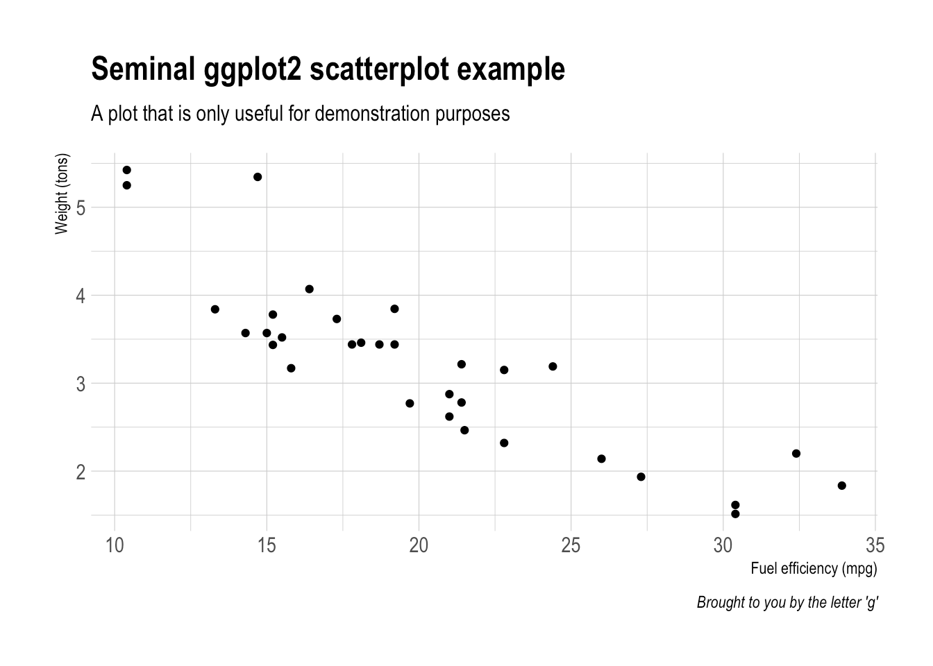

Roboto Condensed

r
ggplot(mtcars, aes(mpg, wt)) +
  geom_point() +
  labs(x="Fuel efficiency (mpg)", y="Weight (tons)",
       title="Seminal ggplot2 scatterplot example",
       subtitle="A plot that is only useful for demonstration purposes",
       caption="Brought to you by the letter 'g'") +
  themeipsumrc()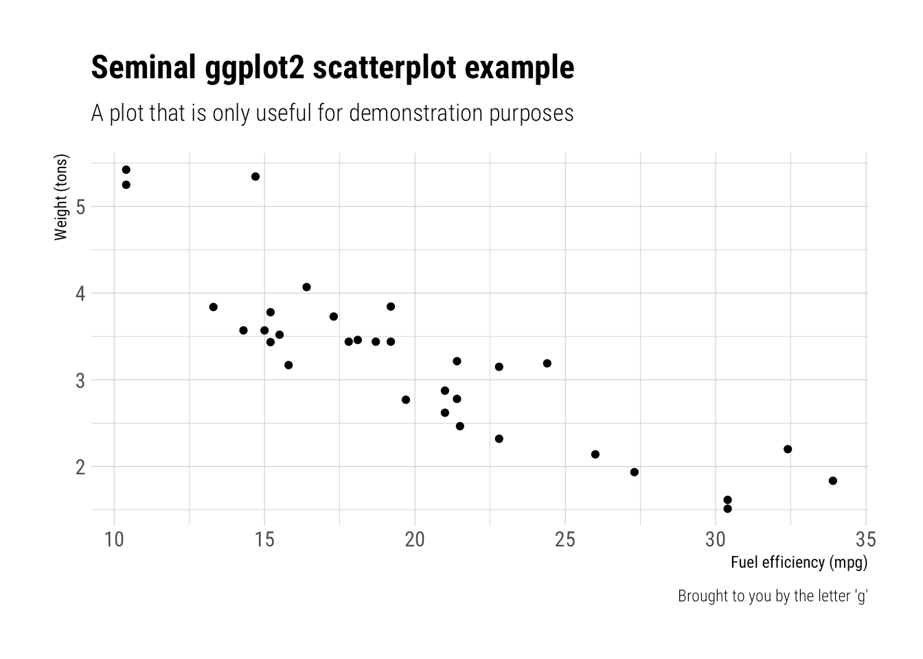

New FT Theme!

r
ggplot(mtcars, aes(mpg, wt)) +
  geompoint(color = ftcols$yellow) +
  labs(x="Fuel efficiency (mpg)", y="Weight (tons)",
       title="Seminal ggplot2 scatterplot example",
       subtitle="A plot that is only useful for demonstration purposes",
       caption="Brought to you by the letter 'g'") +
  themeftrc()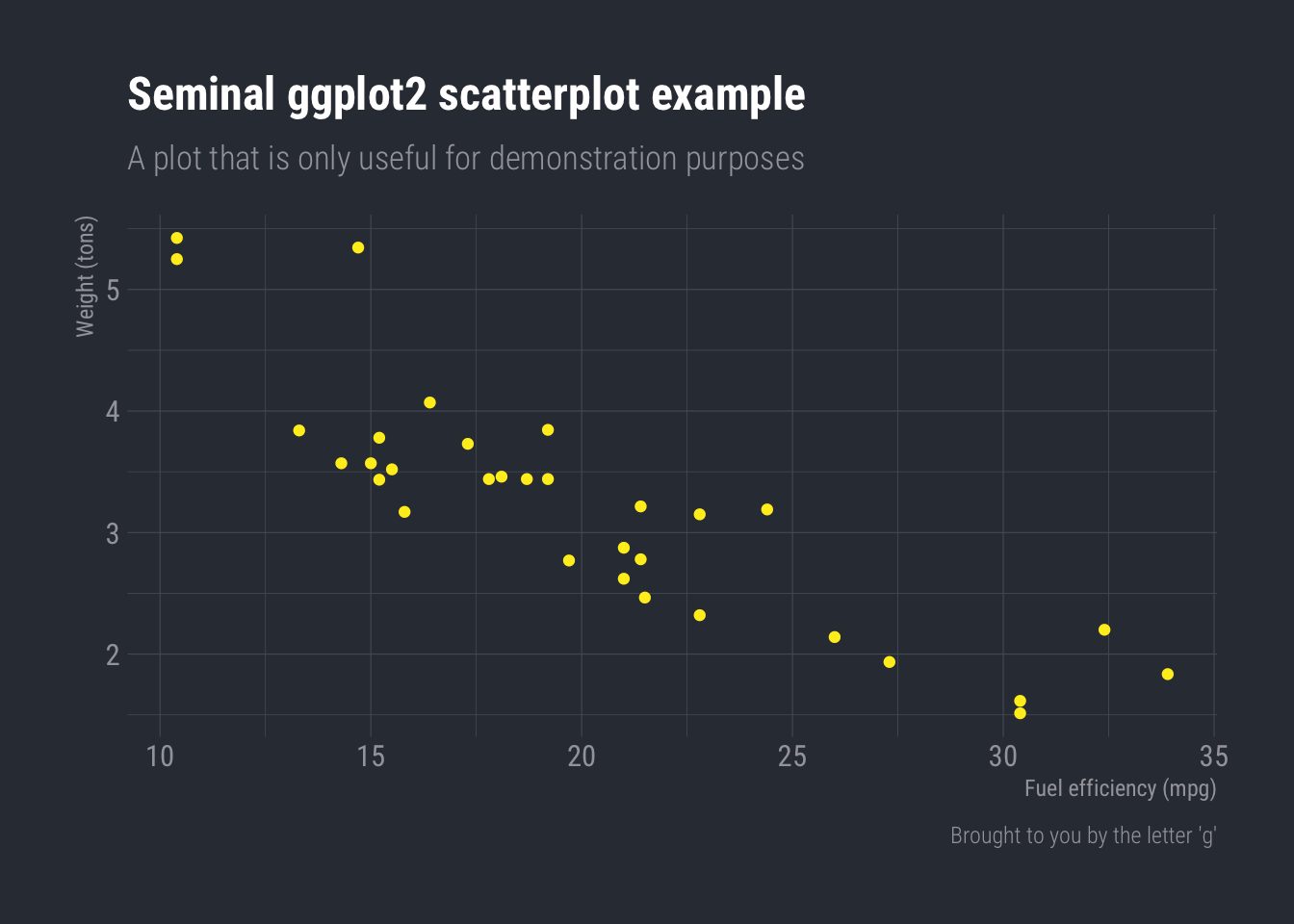

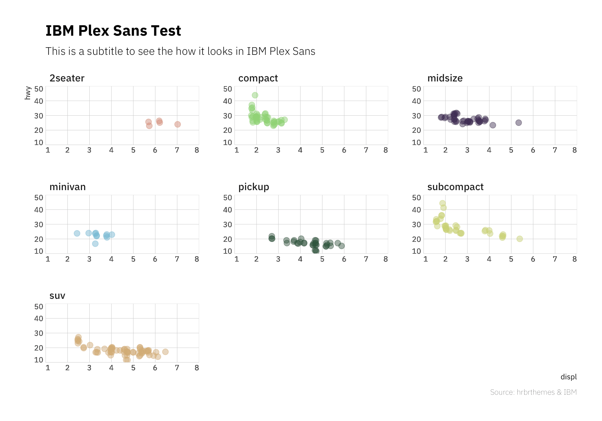
IBM Plex Sans

r
ggplot(mpg, aes(displ, hwy)) +
  geom_jitter(aes(color=class, fill=class), size=3, shape=21, alpha=1/2) +
  scalexcontinuous(expand=c(0,0), limits=c(1, 8), breaks=1:8) +
  scaleycontinuous(expand=c(0,0), limits=c(10, 50)) +
  scalecoloripsum() +
  scalefillipsum() +
  facet_wrap(~class, scales="free") +
  labs(
    title="IBM Plex Sans Test",
    subtitle="This is a subtitle to see the how it looks in IBM Plex Sans",
    caption="Source: hrbrthemes & IBM"
  ) +
  themeipsumps(grid="XY", axis="xy") +
  theme(legend.position="none") -> gg
flush_ticks(gg) 
theme(axis.text.x=element_text(hjust=c(0, rep(0.5, 6), 1))) +
 theme(axis.text.y=element_text(vjust=c(0, rep(0.5, 3), 1)))

Scales (Color/Fill)

r
ggplot(mtcars, aes(mpg, wt)) +
  geom_point(aes(color=factor(carb))) +
  labs(x="Fuel efficiency (mpg)", y="Weight (tons)",
       title="Seminal ggplot2 scatterplot example",
       subtitle="A plot that is only useful for demonstration purposes",
       caption="Brought to you by the letter 'g'") +
  scalecoloripsum() +
  themeipsumrc()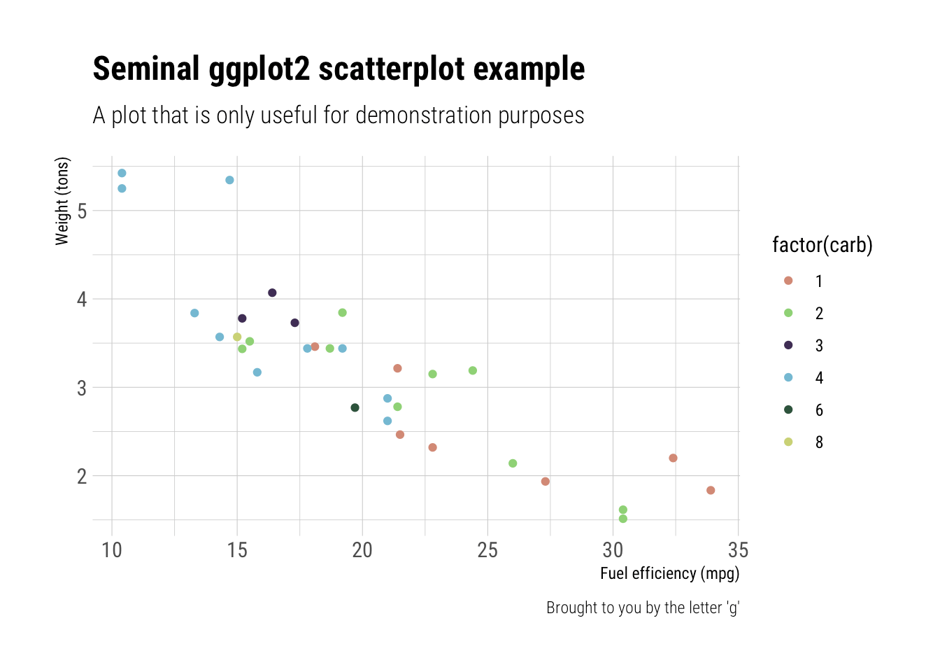

Scales (Axis)

r
count(mpg, class) %>%
  mutate(pct=n/sum(n)) %>%
  ggplot(aes(class, pct)) +
  geom_col() +
  scaleypercent() +
  labs(x="Fuel efficiency (mpg)", y="Weight (tons)",
       title="Seminal ggplot2 column chart example with percents",
       subtitle="A plot that is only useful for demonstration purposes",
       caption="Brought to you by the letter 'g'") +
  theme_ipsum(grid="Y")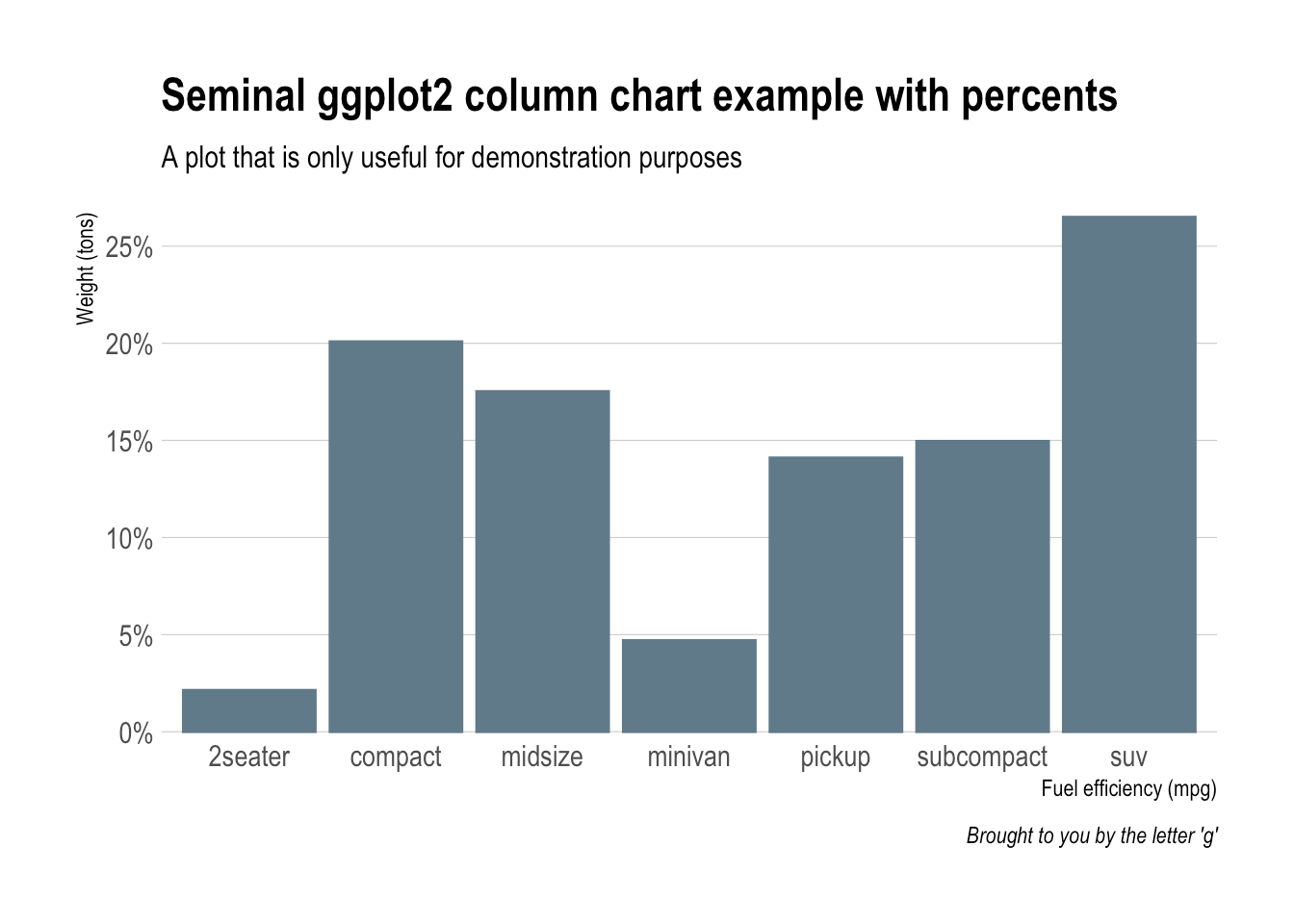

r
ggplot(uspopage, aes(x=Year, y=Thousands, fill=AgeGroup)) +
  geom_area() +
  scalefillipsum() +
  scalexcontinuous(expand=c(0,0)) +
  scaleycomma() +
  labs(title="Age distribution of population in the U.S., 1900-2002",
       subtitle="Example data from the R Graphics Cookbook",
       caption="Source: R Graphics Cookbook") +
  themeipsumrc(grid="XY") +
  theme(axis.text.x=element_text(hjust=c(0, 0.5, 0.5, 0.5, 1))) +
  theme(legend.position="bottom")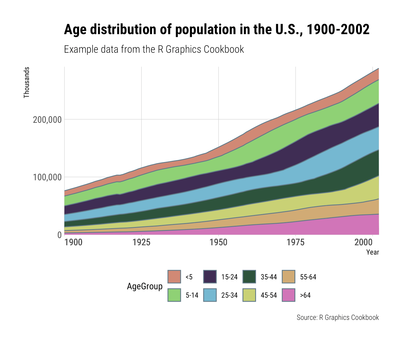

r
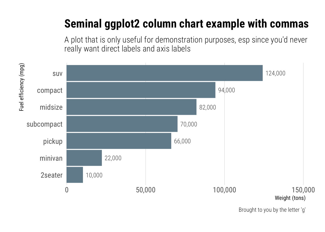
updategeomfontdefaults(fontrc_light)
count(mpg, class) %>%   mutate(n=n*2000) %>%   arrange(n) %>%   mutate(class=factor(class, levels=class)) %>%   ggplot(aes(class, n)) +   geom_col() +   geomtext(aes(label=scales::comma(n)), hjust=0, nudgey=2000) +   scaleycomma(limits=c(0,150000)) +   coord_flip() +   labs(x="Fuel efficiency (mpg)", y="Weight (tons)",        title="Seminal ggplot2 column chart example with commas",        subtitle="A plot that is only useful for demonstration purposes, esp since you'd never\nreally want direct labels and axis labels",        caption="Brought to you by the letter 'g'") +   themeipsumrc(grid="X")

Spellcheck ggplot2 labels

r
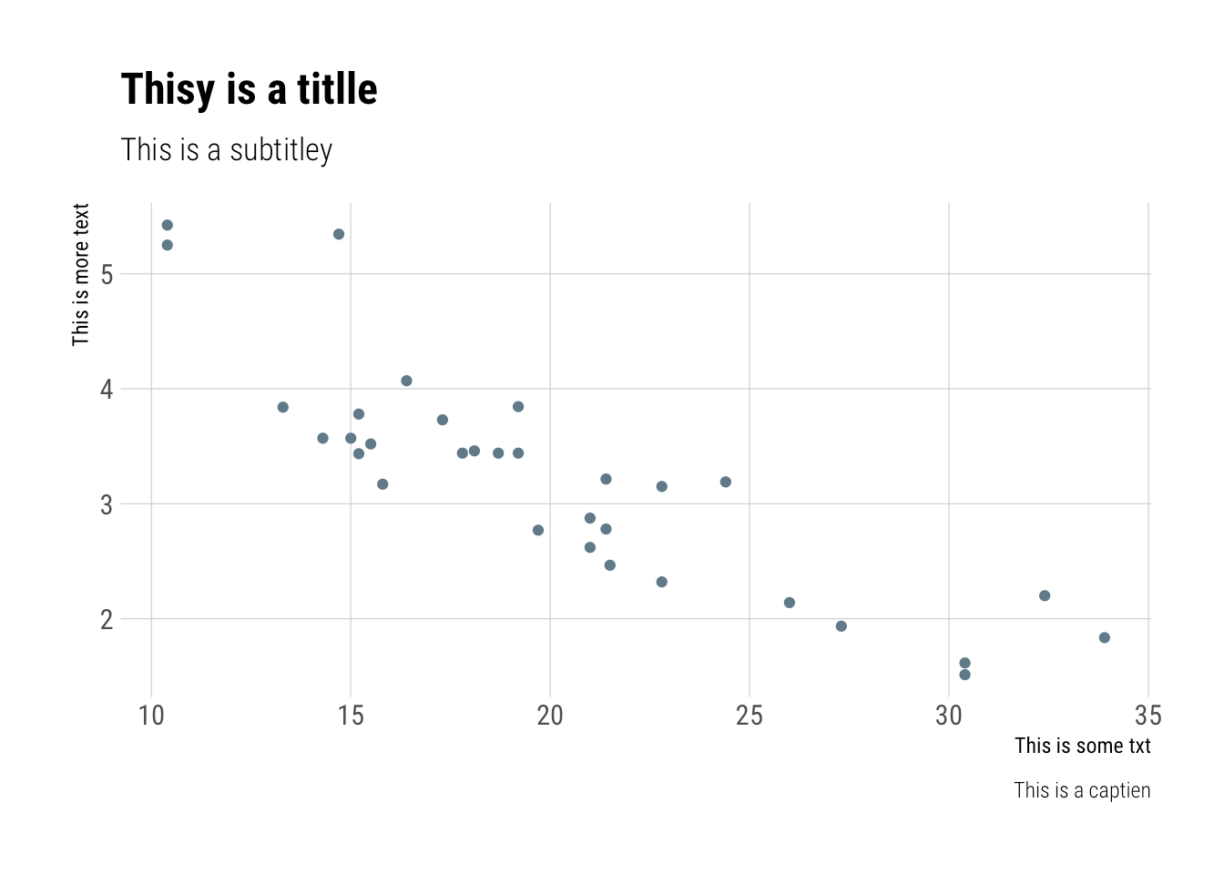
df <- data.frame(x=c(20, 25, 30), y=c(4, 4, 4), txt=c("One", "Two", "Three"))
ggplot(mtcars, aes(mpg, wt)) +   geom_point() +   labs(x="This is some txt", y="This is more text",        title="Thisy is a titlle",        subtitle="This is a subtitley",        caption="This is a captien") +   themeipsumrc(grid="XY") -> gg
gg_check(gg) 
Possible misspelled words in [title]: (Thisy, titlle)
 Possible misspelled words in [subtitle]: (subtitley)
 Possible misspelled words in [caption]: (captien)

Flexoki Color Scales

The Flexoki color system provides both discrete and continuous color scales in light and dark variants.

r
Discrete colors example with light variant
ggplot(mpg, aes(class, fill=class)) +
  geom_bar() +
  labs(title="Flexoki Light Colors",
       subtitle="Discrete color scale example",
       caption="Using scalefillflexoki_light()") +
  theme_ipsum() +
  scalefillflexoki_light() +
  theme(legend.position="none")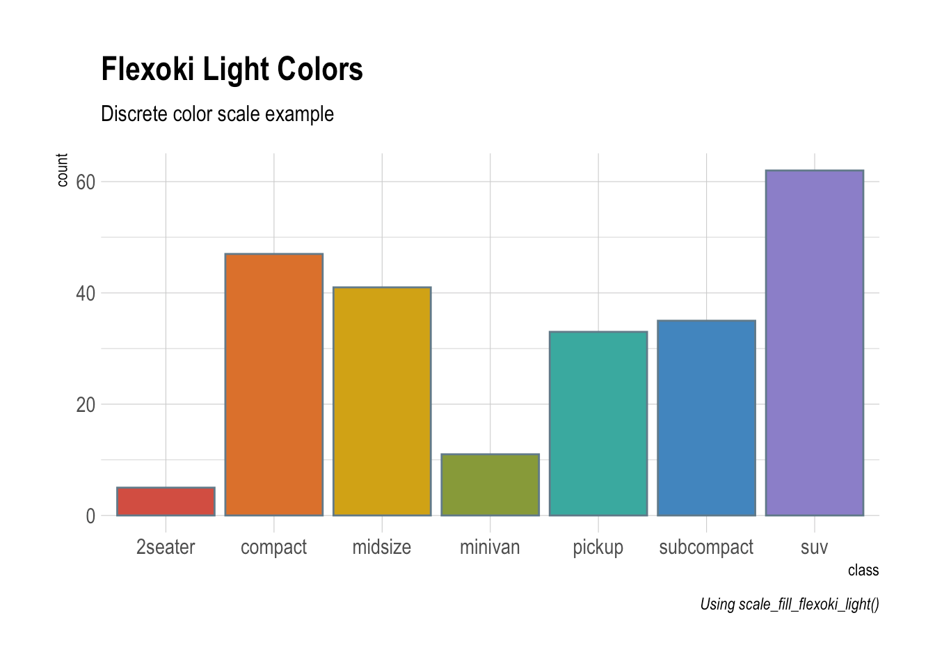

r
Dark variant with points
ggplot(mpg, aes(displ, hwy, color=class)) +
  geom_point(size=3) +
  labs(title="Flexoki Dark Colors",
       subtitle="Another discrete color example",
       caption="Using scalecolorflexoki_dark()") +
  themeipsumrc() +
  scalecolorflexoki_dark()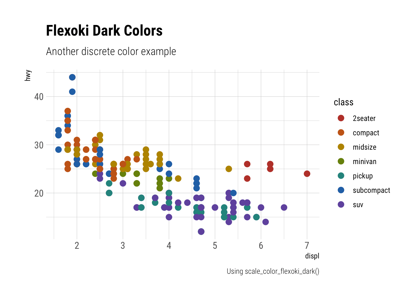

r
library(patchwork)
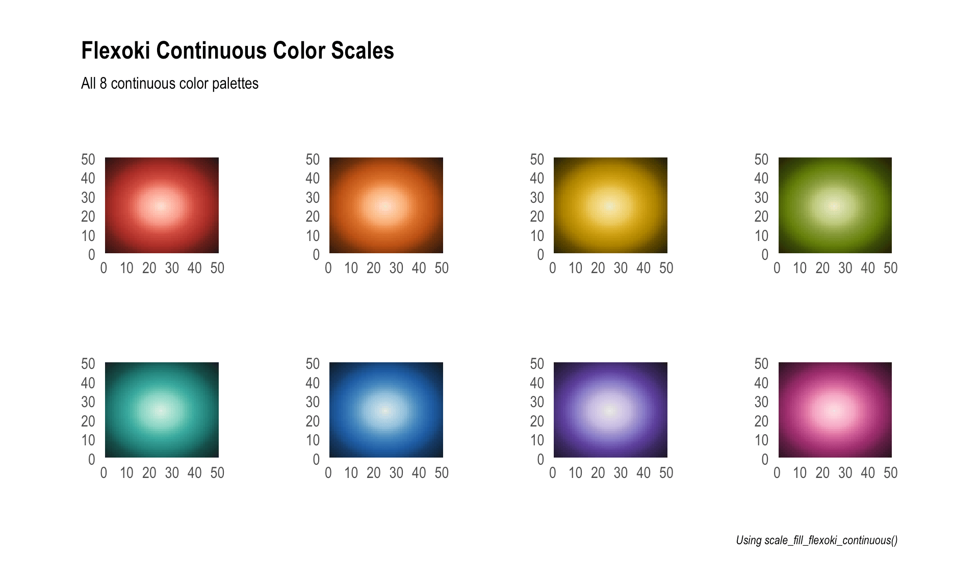
data.frame(   x = rep(1:50, 50),   y = rep(1:50, each=50),   z = sqrt((rep(1:50, 50)-25)^2 + (rep(1:50, each=50)-25)^2) ) -> grad_df
names(flexoki_dark) |>    map(\(.p) {     ggplot(grad_df, aes(x, y, fill=z)) +       geom_tile() +       scalefillflexoki_continuous(palette = .p) +       labs(         x = NULL, y = NULL       ) +       theme_ipsum(grid="") +       theme(legend.position = "none")   }) |>    do.call(what = "wrap_plots") +   plot_layout(ncol = 4) +   plot_annotation(     title="Flexoki Continuous Color Scales",     subtitle="All 8 continuous color palettes",     caption="Using scalefillflexoki_continuous()",     theme = theme_ipsum(grid="")   )

Bit12 Color Scales

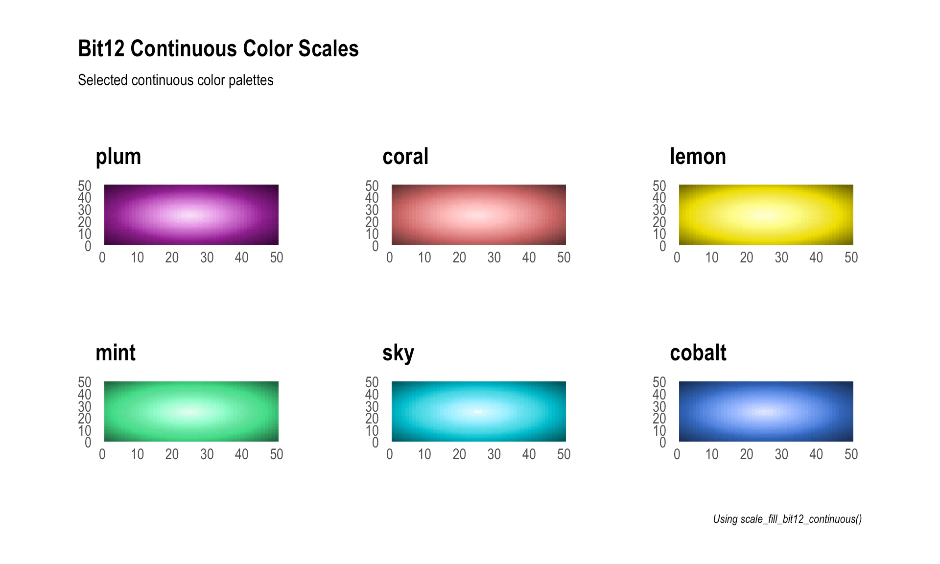
The Bit12 color system provides a set of 12 distinct colors optimized for data visualization.

r
Discrete colors example
ggplot(mpg, aes(class, fill=class)) +
  geom_bar() +
  labs(title="Bit12 Color Palette",
       subtitle="A vibrant 12-color categorical palette",
       caption="Using scalefillbit12()") +
  theme_ipsum() +
  scalefillbit12() +
  theme(legend.position="none")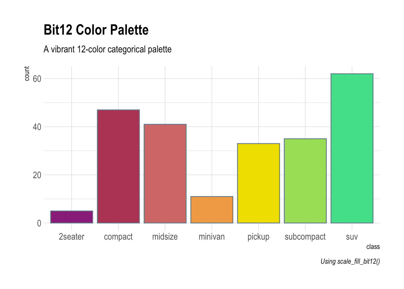

r
library(patchwork)
Taking a subset of the palette for this example
names(bit12)[c(1,3,5,7,9,11)] |> 
  map(\(.p) {
    ggplot(grad_df, aes(x, y, fill=z)) +
      geom_tile() +
      scalefillbit12_continuous(palette = .p) +
      labs(
        x = NULL, y = NULL, title = .p
      ) +
      theme_ipsum(grid="") +
      theme(legend.position = "none")
  }) |> 
  do.call(what = "wrap_plots") +
  plot_layout(ncol = 3) +
  plot_annotation(
    title="Bit12 Continuous Color Scales",
    subtitle="Selected continuous color palettes",
    caption="Using scalefillbit12_continuous()",
    theme = theme_ipsum(grid="")
  )

hrbrthemes Metrics

| Lang | \# Files | (%) | LoC | (%) | Blank lines | (%) | \# Lines | (%) | |:-----|---------:|-----:|-----:|-----:|------------:|----:|---------:|----:| | R | 23 | 0.44 | 1840 | 0.46 | 339 | 0.5 | 1290 | 0.5 | | SVG | 2 | 0.04 | 150 | 0.04 | 0 | 0.0 | 0 | 0.0 | | JSON | 1 | 0.02 | 15 | 0.00 | 0 | 0.0 | 0 | 0.0 | | SUM | 26 | 0.50 | 2005 | 0.50 | 339 | 0.5 | 1290 | 0.5 |

{cloc} 📦 metrics for hrbrthemes