PyIndicators

PyIndicators is a powerful and user-friendly Python library for financial technical analysis indicators, metrics and helper functions. Written entirely in Python, it requires no external dependencies, ensuring seamless integration and ease of use.

Marketplace

We support Finterion as our go-to marketplace for quantitative trading and trading bots.

Works with the Investing Algorithm Framework

PyIndicators works natively with the Investing Algorithm Framework for creating trading bots. All indicators accept the DataFrame format returned by the framework, so you can go from market data to trading signals without any conversion or glue code.

from investingalgorithmframework import download
from pyindicators import ema, rsi, supertrend
Download data directly into a DataFrame
df = download(
    symbol="btc/eur",
    market="binance",
    time_frame="1d",
    start_date="2024-01-01",
    end_date="2024-06-01",
    pandas=True,
    save=True,
    storage_path="./data"
)
Apply indicators — no conversion needed
df = ema(df, source_column="Close", period=200)
df = rsi(df, source_column="Close")
df = supertrend(df, atr_length=10, factor=3.0)

Installation

PyIndicators can be installed using pip:

pip install pyindicators

Features

• Native Python implementation, no external dependencies needed except for Polars or Pandas
• Dataframe first approach, with support for both pandas dataframes and polars dataframes
• Supports python version 3.10 and above.
• Trend indicators

* Weighted Moving Average (WMA) * Simple Moving Average (SMA) * Exponential Moving Average (EMA) * Zero-Lag EMA Envelope (ZLEMA) * EMA Trend Ribbon * SuperTrend * SuperTrend Clustering * Pulse Mean Accelerator (PMA) * Volume Weighted Trend (VWT)

• Momentum and Oscillators

* Moving Average Convergence Divergence (MACD) * Relative Strength Index (RSI) * Relative Strength Index Wilders method (Wilders RSI) * Williams %R * Average Directional Index (ADX) * Stochastic Oscillator (STO) * Momentum Confluence

• Volatility indicators

* Bollinger Bands (BB) * Bollinger Bands Overshoot * Average True Range (ATR) * Moving Average Envelope (MAE) * Nadaraya-Watson Envelope (NWE)

• Support and Resistance

* Fibonacci Retracement * Golden Zone * Golden Zone Signal * Fair Value Gap (FVG) * Order Blocks * Breaker Blocks * Mitigation Blocks * Rejection Blocks * Optimal Trade Entry (OTE) * Market Structure Break * Market Structure CHoCH/BOS * Liquidity Sweeps * Buyside & Sellside Liquidity * Pure Price Action Liquidity Sweeps * Liquidity Pools * Liquidity Levels / Voids (VP) * Internal & External Liquidity Zones * Premium / Discount Zones * Trendline Breakout Navigator

• Pattern recognition

* Detect Peaks * Detect Bullish Divergence * Detect Bearish Divergence

• Indicator helpers

* Crossover * Is Crossover * Crossunder * Is Crossunder * Is Downtrend * Is Uptrend * hasanylowerthenthreshold

Indicators

Trend Indicators

Indicators that help to determine the direction of the market (uptrend, downtrend, or sideways) and confirm if a trend is in place.

Weighted Moving Average (WMA)

A Weighted Moving Average (WMA) is a type of moving average that assigns greater importance to recent data points compared to older ones. This makes it more responsive to recent price changes compared to a Simple Moving Average (SMA), which treats all data points equally. The WMA does this by using linear weighting, where the most recent prices get the highest weight, and weights decrease linearly for older data points.

def wma(
    data: Union[PandasDataFrame, PolarsDataFrame],
    source_column: str,
    period: int,
    result_column: Optional[str] = None
) -> Union[PandasDataFrame, PolarsDataFrame]:

Example

from investingalgorithmframework import download
from pyindicators import wma
pl_df = download(     symbol="btc/eur",     market="binance",     time_frame="1d",     start_date="2023-12-01",     end_date="2023-12-25",     save=True,     storage_path="./data" ) pd_df = download(     symbol="btc/eur",     market="binance",     time_frame="1d",     start_date="2023-12-01",     end_date="2023-12-25",     pandas=True,     save=True,     storage_path="./data" )
Calculate SMA for Polars DataFrame
pldf = wma(pldf, sourcecolumn="Close", period=200, resultcolumn="WMA_200")
pl_df.show(10)
Calculate SMA for Pandas DataFrame
pddf = wma(pddf, sourcecolumn="Close", period=200, resultcolumn="WMA_200")
pd_df.tail(10)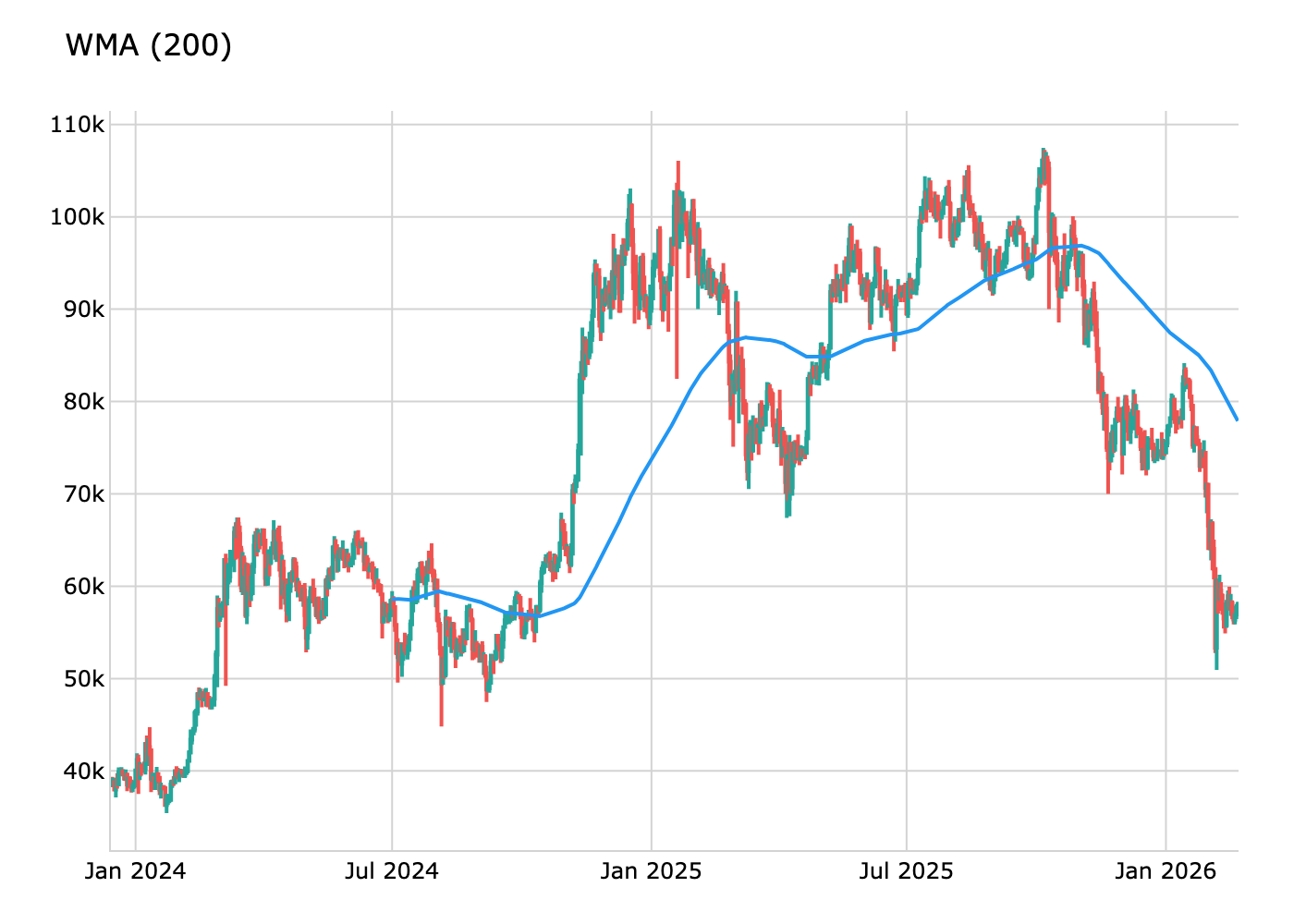

Simple Moving Average (SMA)

A Simple Moving Average (SMA) is the average of the last N data points, recalculated as new data comes in. Unlike the Weighted Moving Average (WMA), SMA treats all values equally, giving them the same weight.

def sma(
    data: Union[PdDataFrame, PlDataFrame],
    source_column: str,
    period: int,
    result_column: str = None,
) -> Union[PdDataFrame, PlDataFrame]:

Example

from investingalgorithmframework import download
from pyindicators import sma
pl_df = download(     symbol="btc/eur",     market="binance",     time_frame="1d",     start_date="2023-12-01",     end_date="2023-12-25",     save=True,     storage_path="./data" ) pd_df = download(     symbol="btc/eur",     market="binance",     time_frame="1d",     start_date="2023-12-01",     end_date="2023-12-25",     pandas=True,     save=True,     storage_path="./data" )
Calculate SMA for Polars DataFrame
pldf = sma(pldf, sourcecolumn="Close", period=200, resultcolumn="SMA_200")
pl_df.show(10)
Calculate SMA for Pandas DataFrame
pddf = sma(pddf, sourcecolumn="Close", period=200, resultcolumn="SMA_200")
pd_df.tail(10)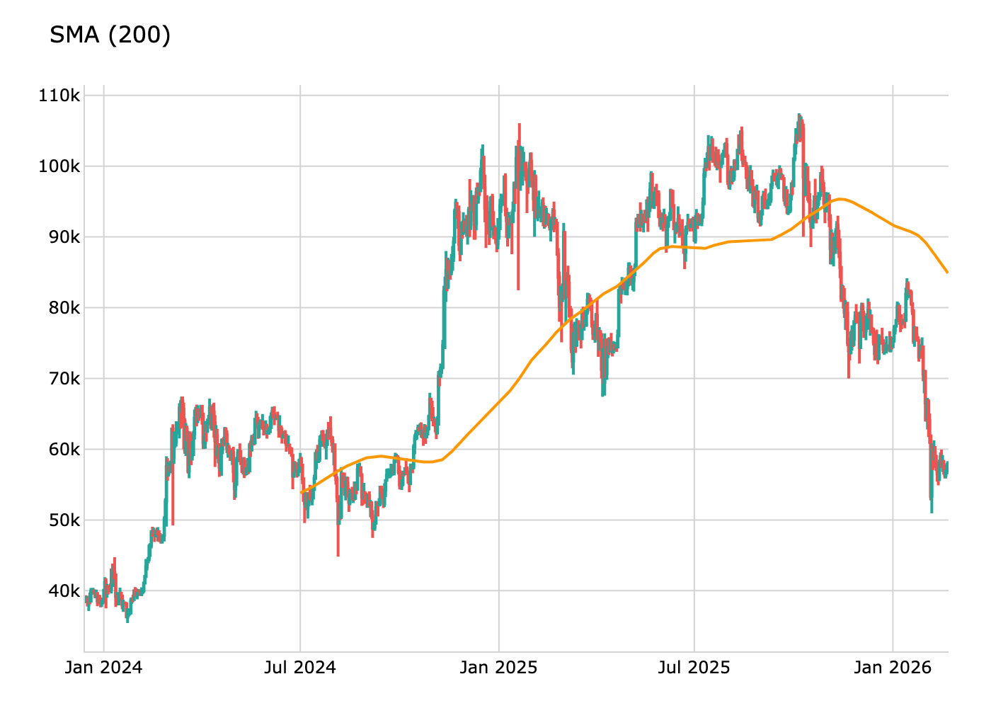

Exponential Moving Average (EMA)

The Exponential Moving Average (EMA) is a type of moving average that gives more weight to recent prices, making it more responsive to price changes than a Simple Moving Average (SMA). It does this by using an exponential decay where the most recent prices get exponentially more weight.

def ema(
    data: Union[PdDataFrame, PlDataFrame],
    source_column: str,
    period: int,
    result_column: str = None,
) -> Union[PdDataFrame, PlDataFrame]:

Example

from investingalgorithmframework import download
from pyindicators import ema
pl_df = download(     symbol="btc/eur",     market="binance",     time_frame="1d",     start_date="2023-12-01",     end_date="2023-12-25",     save=True,     storage_path="./data" ) pd_df = download(     symbol="btc/eur",     market="binance",     time_frame="1d",     start_date="2023-12-01",     end_date="2023-12-25",     pandas=True,     save=True,     storage_path="./data" )
Calculate EMA for Polars DataFrame
pldf = ema(pldf, sourcecolumn="Close", period=200, resultcolumn="EMA_200")
pl_df.show(10)
Calculate EMA for Pandas DataFrame
pddf = ema(pddf, sourcecolumn="Close", period=200, resultcolumn="EMA_200")
pd_df.tail(10)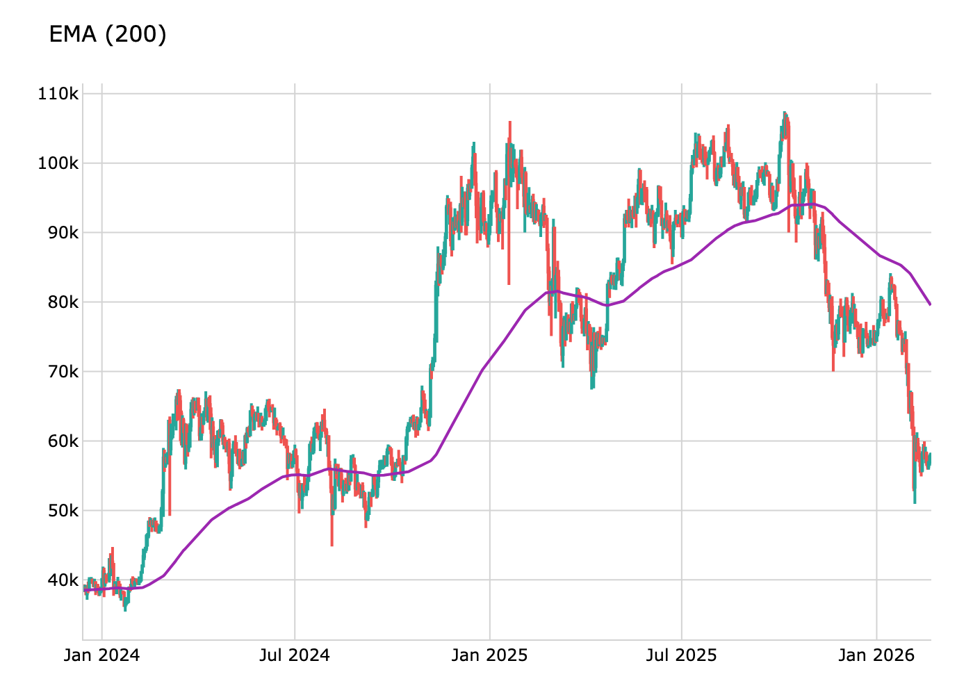

Zero-Lag EMA Envelope (ZLEMA)

The Zero-Lag EMA Envelope combines a Zero-Lag Exponential Moving Average (ZLEMA) with ATR-based bands and multi-bar swing confirmation. The ZLEMA compensates for the inherent lag of a standard EMA by using a lag-compensated source (close + (close - close[lag])). Trend state is confirmed when multiple consecutive bars close beyond a band while the ZLEMA slope agrees.

Calculation:

• lag = floor((length - 1) / 2)
• compensated = close + (close - close[lag])
• ZLEMA = EMA(compensated, length)
• Upper = ZLEMA + ATR × mult
• Lower = ZLEMA - ATR × mult
• Bull: close > Upper for N bars AND ZLEMA rising
• Bear: close < Lower for N bars AND ZLEMA falling

def zerolagema_envelope(     data: Union[PdDataFrame, PlDataFrame],     source_column: str = 'Close',     length: int = 200,     mult: float = 2.0,     atr_length: int = 21,     confirm_bars: int = 2,     uppercolumn: str = 'zlemaupper',     lowercolumn: str = 'zlemalower',     middlecolumn: str = 'zlemamiddle',     trendcolumn: str = 'zlematrend',     signalcolumn: str = 'zlemasignal', ) -> Union[PdDataFrame, PlDataFrame]:

Example

from investingalgorithmframework import download
from pyindicators import zerolagema_envelope
pl_df = download(     symbol="btc/eur",     market="binance",     time_frame="1d",     start_date="2023-12-01",     end_date="2023-12-25",     save=True,     storage_path="./data" ) pd_df = download(     symbol="btc/eur",     market="binance",     time_frame="1d",     start_date="2023-12-01",     end_date="2023-12-25",     pandas=True,     save=True,     storage_path="./data" )
Calculate Zero-Lag EMA Envelope for Polars DataFrame
pldf = zerolagemaenvelope(pldf, sourcecolumn="Close", length=200, mult=2.0)
pl_df.show(10)
Calculate Zero-Lag EMA Envelope for Pandas DataFrame
pddf = zerolagemaenvelope(pddf, sourcecolumn="Close", length=200, mult=2.0)
pd_df.tail(10)

EMA Trend Ribbon

The EMA Trend Ribbon uses 9 Exponential Moving Averages with increasing periods to visualise trend strength and direction. At each bar the slope of every EMA is checked over a smoothing window; when a threshold number of EMAs agree on direction (default 7 out of 9) the trend is classified as bullish or bearish.

Calculation:

• Compute 9 EMAs with periods [8, 14, 20, 26, 32, 38, 44, 50, 60]
• An EMA is "rising" when EMA[t] >= EMA[t - smoothing_period]
• bullish_count = number of rising EMAs
• bearish_count = number of falling EMAs
• Trend = 1 if bullishcount >= threshold, -1 if bearishcount >= threshold, else 0

def ematrendribbon(     data: Union[PdDataFrame, PlDataFrame],     source_column: str = 'Close',     ema_lengths: Optional[List[int]] = None,  # default [8,14,20,26,32,38,44,50,60]     smoothing_period: int = 2,     threshold: int = 7,     trendcolumn: str = 'emaribbon_trend',     bullishcountcolumn: str = 'emaribbonbullish_count',     bearishcountcolumn: str = 'emaribbonbearish_count',     emacolumnprefix: str = 'ema_ribbon', ) -> Union[PdDataFrame, PlDataFrame]:

Example

from investingalgorithmframework import download
from pyindicators import ematrendribbon
pl_df = download(     symbol="btc/eur",     market="binance",     time_frame="1d",     start_date="2023-12-01",     end_date="2023-12-25",     save=True,     storage_path="./data" ) pd_df = download(     symbol="btc/eur",     market="binance",     time_frame="1d",     start_date="2023-12-01",     end_date="2023-12-25",     pandas=True,     save=True,     storage_path="./data" )
Calculate EMA Trend Ribbon for Polars DataFrame
pldf = ematrendribbon(pldf, source_column="Close")
pl_df.show(10)
Calculate EMA Trend Ribbon for Pandas DataFrame
pddf = ematrendribbon(pddf, source_column="Close")
pd_df.tail(10)

SuperTrend

The SuperTrend indicator uses a fixed ATR multiplier factor to create a trend-following trailing stop. When the price is above the SuperTrend line the trend is bullish; when below, bearish. Trend changes generate buy/sell signals.

def supertrend(
    data: Union[PdDataFrame, PlDataFrame],
    atr_length: int = 10,
    factor: float = 3.0
) -> Union[PdDataFrame, PlDataFrame]:

Returns the following columns:

• supertrend: The SuperTrend trailing stop value
• supertrend_trend: Current trend (1=bullish, 0=bearish)
• supertrend_upper: Upper band
• supertrend_lower: Lower band
• supertrend_signal: 1=buy signal, -1=sell signal, 0=no signal

Example

from investingalgorithmframework import download
from pyindicators import supertrend
pd_df = download(     symbol="btc/eur",     market="binance",     time_frame="1d",     start_date="2023-12-01",     end_date="2023-12-25",     pandas=True,     save=True,     storage_path="./data" )
Calculate SuperTrend
pddf = supertrend(pddf, atr_length=10, factor=3.0)
pd_df.tail(10)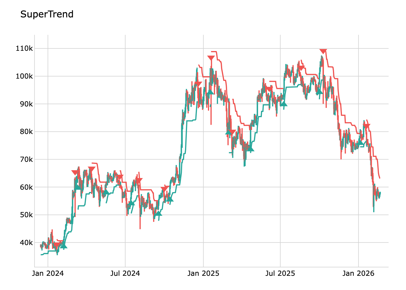

SuperTrend Clustering

The SuperTrend Clustering indicator uses K-means clustering to optimize the ATR multiplier factor for the SuperTrend calculation. It computes multiple SuperTrend variations with different factors, evaluates their performance, and clusters them into "best", "average", and "worst" groups. The best-performing factor is then used to generate an adaptive trailing stop with buy/sell signals.

def supertrend_clustering(
    data: Union[PdDataFrame, PlDataFrame],
    atr_length: int = 10,
    min_mult: float = 1.0,
    max_mult: float = 5.0,
    step: float = 0.5,
    perf_alpha: float = 10.0,
    from_cluster: str = 'best',
    max_iter: int = 1000,
    max_data: int = 10000
) -> Union[PdDataFrame, PlDataFrame]:

Returns the following columns:

• supertrend: The optimized SuperTrend trailing stop
• supertrend_trend: Current trend (1=bullish, 0=bearish)
• supertrend_ama: Adaptive moving average of SuperTrend
• supertrendperfidx: Performance index (0–1 scale)
• supertrend_factor: Currently used ATR factor
• supertrend_signal: 1=buy signal, -1=sell signal, 0=no signal

Example

from investingalgorithmframework import download
from pyindicators import supertrendclustering, getsupertrend_stats
pd_df = download(     symbol="btc/eur",     market="binance",     time_frame="1d",     start_date="2023-12-01",     end_date="2023-12-25",     pandas=True,     save=True,     storage_path="./data" )
Calculate SuperTrend Clustering
pddf = supertrendclustering(
    pd_df,
    atr_length=14,
    min_mult=2.0,
    max_mult=6.0,
    step=0.5,
    perf_alpha=14.0,
    from_cluster='best',
    max_data=500
)
Get statistics
stats = getsupertrendstats(pd_df)
print(stats)
pd_df.tail(10)

Pulse Mean Accelerator (PMA)

The Pulse Mean Accelerator is a trend-following overlay indicator translated from the Pine Script® by MisinkoMaster. It adds a volatility- and momentum-scaled acceleration offset to a base moving average. The acceleration accumulates over a configurable lookback: bars where source momentum exceeds MA momentum push the PMA further from the MA, while bars where the MA leads source momentum pull it back. Multiple MA types (RMA, SMA, EMA, WMA, DEMA, TEMA, HMA), volatility measures (ATR, Standard Deviation, MAD), and smoothing modes are supported.

Parameters:

| Parameter | Type | Default | Description | |---|---|---|---| | source_column | str | "Close" | Source price column | | ma_type | str | "RMA" | MA type: RMA, SMA, EMA, WMA, DEMA, TEMA, HMA | | ma_length | int | 20 | Lookback for the base moving average | | accel_lookback | int | 32 | Bars over which acceleration is accumulated | | max_accel | float | 0.2 | Maximum absolute acceleration factor | | volatility_type | str | "Standard Deviation" | Volatility: ATR, Standard Deviation, MAD | | smooth_type | str | "Double Moving Average" | Smoothing: NONE, Exponential, Extra Moving Average, Double Moving Average | | use_confirmation | bool | True | Require combined PMA+MA momentum to confirm trend flips |

Output columns: pma, pmama, pmatrend, pmalong, pmashort, pma_acceleration

import pandas as pd
from pyindicators import (
    pulsemeanaccelerator,
    pulsemeanaccelerator_signal,
    getpulsemeanacceleratorstats,
)
--- With pandas ---
df = pd.read_csv("data.csv")
df = pulsemeanaccelerator(
    df,
    ma_type="RMA",
    ma_length=20,
    accel_lookback=32,
    max_accel=0.2,
    volatility_type="Standard Deviation",
    smooth_type="Double Moving Average",
    use_confirmation=True,
)
df = pulsemeanaccelerator_signal(df)
stats = getpulsemeanacceleratorstats(df)
print(stats)
df[["Close", "pma", "pmama", "pmatrend", "pmalong", "pmashort"]].tail(10)

Volume Weighted Trend (VWT)

The Volume Weighted Trend indicator uses a Volume Weighted Moving Average (VWMA) with ATR-based volatility bands to determine trend direction. Based on the "Volume Weighted Trend [QuantAlgo]" concept. The VWMA serves as the trend baseline, while upper and lower bands (VWMA +/- ATR * multiplier) define breakout thresholds. The trend flips bullish when price closes above the upper band and bearish when price closes below the lower band.

def volumeweightedtrend(
    df: Union[PdDataFrame, PlDataFrame],
    vwma_length: int = 34,
    atr_multiplier: float = 1.5,
    high_column: str = "High",
    low_column: str = "Low",
    close_column: str = "Close",
    volume_column: str = "Volume",
) -> Union[PdDataFrame, PlDataFrame]:

Returns the following columns:

• vwt_vwma: Volume Weighted Moving Average
• vwt_atr: Average True Range
• vwt_upper: Upper volatility band (VWMA + ATR * multiplier)
• vwt_lower: Lower volatility band (VWMA - ATR * multiplier)
• vwt_trend: Trend direction (+1 bullish, -1 bearish, 0 undefined)
• vwttrendchanged: 1 on bars where trend flipped, 0 otherwise
• vwt_signal: +1 on bullish flip, -1 on bearish flip, 0 otherwise

Example

from investingalgorithmframework import download
from pyindicators import volumeweightedtrend, getvolumeweightedtrendstats
pd_df = download(     symbol="btc/eur",     market="bitvavo",     time_frame="4h",     start_date="2024-01-01",     end_date="2024-04-01",     pandas=True, )
Calculate Volume Weighted Trend
pddf = volumeweightedtrend(pddf, vwmalength=34, atrmultiplier=1.5)
Get summary statistics
stats = getvolumeweightedtrendstats(pd_df)
print(stats)
pddf[["Close", "vwtvwma", "vwtupper", "vwtlower", "vwttrend", "vwtsignal"]].tail(10)

Momentum and Oscillators

Indicators that measure the strength and speed of price movements rather than the direction.

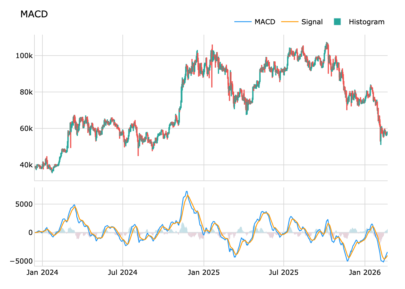
Moving Average Convergence Divergence (MACD)

The Moving Average Convergence Divergence (MACD) is used to identify trend direction, strength, and potential reversals. It is based on the relationship between two Exponential Moving Averages (EMAs) and includes a histogram to visualize momentum.

def macd(
    data: Union[PdDataFrame, PlDataFrame],
    source_column: str,
    short_period: int = 12,
    long_period: int = 26,
    signal_period: int = 9,
    macd_column: str = "macd",
    signalcolumn: str = "macdsignal",
    histogramcolumn: str = "macdhistogram"
) -> Union[PdDataFrame, PlDataFrame]:

Example

from investingalgorithmframework import download
from pyindicators import macd
pl_df = download(     symbol="btc/eur",     market="binance",     time_frame="1d",     start_date="2023-12-01",     end_date="2023-12-25",     save=True,     storage_path="./data" ) pd_df = download(     symbol="btc/eur",     market="binance",     time_frame="1d",     start_date="2023-12-01",     end_date="2023-12-25",     pandas=True,     save=True,     storage_path="./data" )
Calculate MACD for Polars DataFrame
pldf = macd(pldf, sourcecolumn="Close", shortperiod=12, longperiod=26, signalperiod=9)
Calculate MACD for Pandas DataFrame
pddf = macd(pddf, sourcecolumn="Close", shortperiod=12, longperiod=26, signalperiod=9)
pl_df.show(10) pd_df.tail(10)

Relative Strength Index (RSI)

The Relative Strength Index (RSI) is a momentum oscillator that measures the speed and change of price movements. It moves between 0 and 100 and is used to identify overbought or oversold conditions in a market.

def rsi(
    data: Union[pd.DataFrame, pl.DataFrame],
    source_column: str,
    period: int = 14,
    result_column: str = None,
) -> Union[pd.DataFrame, pl.DataFrame]:

Example

from investingalgorithmframework import download
from pyindicators import rsi
pl_df = download(     symbol="btc/eur",     market="binance",     time_frame="1d",     start_date="2023-12-01",     end_date="2023-12-25",     save=True,     storage_path="./data" ) pd_df = download(     symbol="btc/eur",     market="binance",     time_frame="1d",     start_date="2023-12-01",     end_date="2023-12-25",     pandas=True,     save=True,     storage_path="./data" )
Calculate RSI for Polars DataFrame
pldf = rsi(pldf, sourcecolumn="Close", period=14, resultcolumn="RSI_14")
pl_df.show(10)
Calculate RSI for Pandas DataFrame
pddf = rsi(pddf, sourcecolumn="Close", period=14, resultcolumn="RSI_14")
pd_df.tail(10)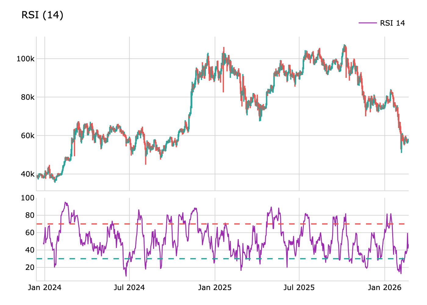

Wilders Relative Strength Index (Wilders RSI)

The Wilders Relative Strength Index (RSI) is a momentum oscillator that measures the speed and change of price movements. It moves between 0 and 100 and is used to identify overbought or oversold conditions in a market. The Wilders RSI uses a different calculation method than the standard RSI.

def wilders_rsi(
    data: Union[pd.DataFrame, pl.DataFrame],
    source_column: str,
    period: int = 14,
    result_column: str = None,
) -> Union[pd.DataFrame, pl.DataFrame]:

Example

from investingalgorithmframework import download
from pyindicators import wilders_rsi
pl_df = download(     symbol="btc/eur",     market="binance",     time_frame="1d",     start_date="2023-12-01",     end_date="2023-12-25",     save=True,     storage_path="./data" ) pd_df = download(     symbol="btc/eur",     market="binance",     time_frame="1d",     start_date="2023-12-01",     end_date="2023-12-25",     pandas=True,     save=True,     storage_path="./data" )
Calculate Wilders RSI for Polars DataFrame
pldf = wildersrsi(pldf, sourcecolumn="Close", period=14, resultcolumn="RSI14")
pl_df.show(10)
Calculate Wilders RSI for Pandas DataFrame
pddf = wildersrsi(pddf, sourcecolumn="Close", period=14, resultcolumn="RSI14")
pd_df.tail(10)

Williams %R

Williams %R (Williams Percent Range) is a momentum indicator used in technical analysis to measure overbought and oversold conditions in a market. It moves between 0 and -100 and helps traders identify potential reversal points.

def willr(
    data: Union[pd.DataFrame, pl.DataFrame],
    period: int = 14,
    result_column: str = None,
    high_column: str = "High",
    low_column: str = "Low",
    close_column: str = "Close"
) -> Union[pd.DataFrame, pl.DataFrame]:

Example

from investingalgorithmframework import download
from pyindicators import willr
pl_df = download(     symbol="btc/eur",     market="binance",     time_frame="1d",     start_date="2023-12-01",     end_date="2023-12-25",     save=True,     storage_path="./data" ) pd_df = download(     symbol="btc/eur",     market="binance",     time_frame="1d",     start_date="2023-12-01",     end_date="2023-12-25",     pandas=True,     save=True,     storage_path="./data" )
pldf = datasource.get_data() pddf = datasource.get_data(pandas=True)
Calculate Williams%R for Polars DataFrame
pldf = willr(pldf, result_column="WILLR")
pl_df.show(10)
Calculate Williams%R for Pandas DataFrame
pddf = willr(pddf, result_column="WILLR")
pd_df.tail(10)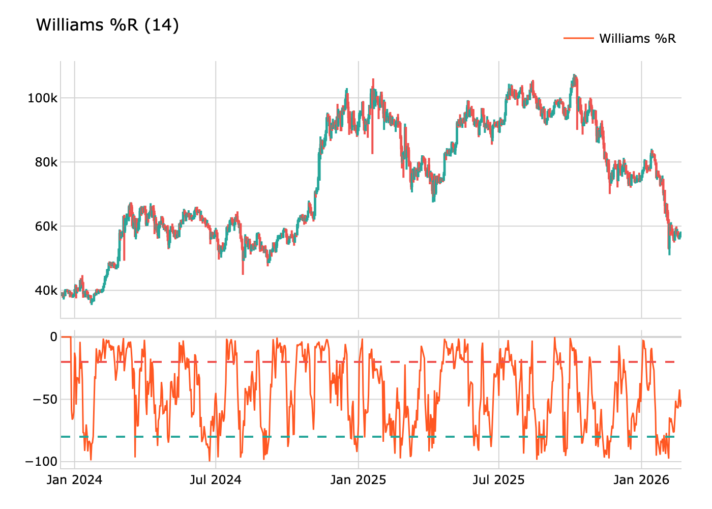

Average Directional Index (ADX)

The Average Directional Index (ADX) is a trend strength indicator that helps traders identify the strength of a trend, regardless of its direction. It is derived from the Positive Directional Indicator (+DI) and Negative Directional Indicator (-DI) and moves between 0 and 100.

def adx(
    data: Union[PdDataFrame, PlDataFrame],
    period=14,
    adxresultcolumn="ADX",
    diplusresult_column="+DI",
    diminusresult_column="-DI",
) -> Union[PdDataFrame, PlDataFrame]:

Example

from investingalgorithmframework import download
from pyindicators import adx
pl_df = download(     symbol="btc/eur",     market="binance",     time_frame="1d",     start_date="2023-12-01",     end_date="2023-12-25",     save=True,     storage_path="./data" ) pd_df = download(     symbol="btc/eur",     market="binance",     time_frame="1d",     start_date="2023-12-01",     end_date="2023-12-25",     pandas=True,     save=True,     storage_path="./data" )
Calculate ADX for Polars DataFrame
pldf = adx(pldf)
pl_df.show(10)
Calculate ADX for Pandas DataFrame
pddf = adx(pddf)
pd_df.tail(10)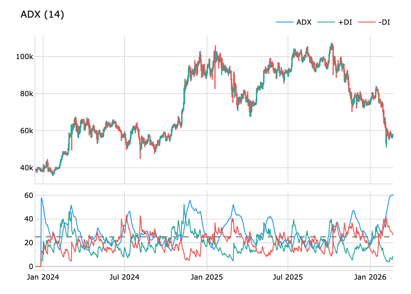

Stochastic Oscillator (STO)

The Stochastic Oscillator (STO) is a momentum indicator that compares a particular closing price of an asset to a range of its prices over a certain period. It is used to identify overbought or oversold conditions in a market. The STO consists of two lines: %K and %D, where %K is the main line and %D is the signal line.

def stochastic_oscillator(
    data: Union[pd.DataFrame, pl.DataFrame],
    high_column: str = "High",
    low_column: str = "Low",
    close_column: str = "Close",
    k_period: int = 14,
    k_slowing: int = 3,
    d_period: int = 3,
    result_column: Optional[str] = None
) -> Union[pd.DataFrame, pl.DataFrame]:

Example

from investingalgorithmframework import download
from pyindicators import stochastic_oscillator
pl_df = download(
    symbol="btc/eur",
    market="binance",
    time_frame="1d",
    start_date="2023-12-01",
    end_date="2023-12-25",
    save=True,
    storage_path="./data"
)
pd_df = download(
    symbol="btc/eur",
    market="binance",
    time_frame="1d",
    start_date="2023-12-01",
    end_date="2023-12-25",
    pandas=True,
    save=True,
    storage_path="./data"
)
Calculate Stochastic Oscillator for Polars DataFrame
pldf = stochasticoscillator(pldf, highcolumn="High", lowcolumn="Low", closecolumn="Close", kperiod=14, kslowing=3, dperiod=3, resultcolumn="STO")
pl_df.show(10)
Calculate Stochastic Oscillator for Pandas DataFrame
pddf = stochasticoscillator(pddf, highcolumn="High", lowcolumn="Low", closecolumn="Close", kperiod=14, kslowing=3, dperiod=3, resultcolumn="STO")
pd_df.tail(10)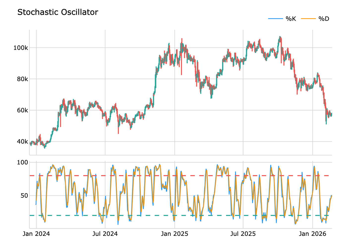

Momentum Confluence

Momentum Confluence is a comprehensive multi-component oscillator that combines multiple technical analysis components to provide a powerful trend following and reversal detection system.

Components:

• Money Flow: Measures buying/selling liquidity entering the market (-100 to +100)
• Thresholds: Dynamic levels showing significant buying/selling activity
• Overflow: Detects excess buying/selling that predicts reversals
• Trend Wave: A highly reactive trend-following oscillator (0-100)
• Real-Time Divergences: Price vs oscillator divergence detection
• Reversal Signals: High-frequency (small dots) and strong (arrows) reversal signals
• Confluence: Combined signal strength from all components (-100 to +100)

def momentum_confluence(     data: Union[PdDataFrame, PlDataFrame],     moneyflowlength: int = 14,     trendwavelength: int = 10,     threshold_mult: float = 1.5,     overflow_threshold: float = 0.8,     divergence_lookback: int = 5,     high_column: str = 'High',     low_column: str = 'Low',     close_column: str = 'Close',     volume_column: str = 'Volume',     ... ) -> Union[PdDataFrame, PlDataFrame]:

Example

from pyindicators import (
    momentum_confluence,
    momentumconfluencesignal,
    getmomentumconfluence_stats
)
Calculate Momentum Confluence
df = momentum_confluence(df)
Generate trading signals
df = momentumconfluencesignal(df)
Get statistics
stats = getmomentumconfluence_stats(df)
print(f"Strong bullish reversals: {stats['strongreversalbullish_count']}")
print(f"Divergences detected: {stats['divergencebullishcount']}")

Output Columns:

• money_flow: Money flow oscillator (-100 to +100)
• mfupperthreshold / mflowerthreshold: Dynamic threshold levels
• overflowbullish / overflowbearish: Excess buying/selling (0 or 1)
• trend_wave: Trend oscillator (0-100)
• trendwavesignal: Trend direction (1=bullish, -1=bearish, 0=neutral)
• divergencebullish / divergencebearish: Divergence detection (0 or 1)
• reversalbullish / reversalbearish: High-frequency reversal signals (0 or 1)
• reversalstrongbullish / reversalstrongbearish: Strong reversal signals (0 or 1)
• confluence: Combined signal strength (-100 to +100)
• mc_trend: Overall trend direction (1=bullish, -1=bearish, 0=neutral)

Signal Values (from momentumconfluencesignal):

• 2: Strong bullish reversal signal
• 1: Bullish confluence
• 0: Neutral
• -1: Bearish confluence
• -2: Strong bearish reversal signal

Volatility indicators

Indicators that measure the rate of price movement, regardless of direction. They help to identify periods of high and low volatility in the market.

Bollinger Bands (BB)

Bollinger Bands are a volatility indicator that consists of a middle band (SMA) and two outer bands (standard deviations). They help traders identify overbought and oversold conditions.

def bollinger_bands(
    data: Union[PdDataFrame, PlDataFrame],
    source_column='Close',
    period=20,
    std_dev=2,
    middlebandcolumnresultcolumn='bollinger_middle',
    upperbandcolumnresultcolumn='bollinger_upper',
    lowerbandcolumnresultcolumn='bollinger_lower'
) -> Union[PdDataFrame, PlDataFrame]:

Example

from investingalgorithmframework import download
from pyindicators import bollinger_bands
pl_df = download(     symbol="btc/eur",     market="binance",     time_frame="1d",     start_date="2023-12-01",     end_date="2023-12-25",     save=True,     storage_path="./data" ) pd_df = download(     symbol="btc/eur",     market="binance",     time_frame="1d",     start_date="2023-12-01",     end_date="2023-12-25",     pandas=True,     save=True,     storage_path="./data" )
Calculate bollinger bands for Polars DataFrame
pldf = bollingerbands(pldf, sourcecolumn="Close")
pl_df.show(10)
Calculate bollinger bands for Pandas DataFrame
pddf = bollingerbands(pddf, sourcecolumn="Close")
pd_df.tail(10)

Bollinger Bands Overshoot

Bollinger Bands Overshoot measures how far the price has exceeded the upper or lower Bollinger Band, expressed as a percentage of the half-band width (distance from middle to upper/lower band). This indicator helps identify extreme price movements and potential mean reversion opportunities.

Calculation:

• When price > upper band (bullish overshoot): ((Price - Upper Band) / (Upper Band - Middle Band)) × 100
• When price < lower band (bearish overshoot): ((Price - Lower Band) / (Middle Band - Lower Band)) × 100
• When price is within bands: 0%

Interpretation:

• Positive values indicate overbought conditions (price above upper band)
• Negative values indicate oversold conditions (price below lower band)
• High overshoots (e.g., 40%) indicate increased risk of mean reversion

def bollinger_overshoot(     data: Union[PdDataFrame, PlDataFrame],     source_column='Close',     period=20,     std_dev=2,     resultcolumn='bollingerovershoot' ) -> Union[PdDataFrame, PlDataFrame]:

Example

from investingalgorithmframework import download
from pyindicators import bollinger_overshoot
pl_df = download(     symbol="btc/eur",     market="binance",     time_frame="1d",     start_date="2023-12-01",     end_date="2023-12-25",     save=True,     storage_path="./data" ) pd_df = download(     symbol="btc/eur",     market="binance",     time_frame="1d",     start_date="2023-12-01",     end_date="2023-12-25",     pandas=True,     save=True,     storage_path="./data" )
Calculate Bollinger Bands Overshoot for Polars DataFrame
pldf = bollingerovershoot(pldf, sourcecolumn="Close")
pl_df.show(10)
Calculate Bollinger Bands Overshoot for Pandas DataFrame
pddf = bollingerovershoot(pddf, sourcecolumn="Close")
pd_df.tail(10)

Average True Range (ATR)

The Average True Range (ATR) is a volatility indicator that measures the average range between the high and low prices over a specified period. It helps traders identify potential price fluctuations and adjust their strategies accordingly.

def atr(
    data: Union[PdDataFrame, PlDataFrame],
    source_column="Close",
    period=14,
    result_column="ATR"
) -> Union[PdDataFrame, PlDataFrame]:

Example

from investingalgorithmframework import download
from pyindicators import atr
pl_df = download(     symbol="btc/eur",     market="binance",     time_frame="1d",     start_date="2023-12-01",     end_date="2023-12-25",     save=True,     storage_path="./data" ) pd_df = download(     symbol="btc/eur",     market="binance",     time_frame="1d",     start_date="2023-12-01",     end_date="2023-12-25",     pandas=True,     save=True,     storage_path="./data" )
Calculate average true range for Polars DataFrame
pldf = atr(pldf, source_column="Close")
pl_df.show(10)
Calculate average true range for Pandas DataFrame
pddf = atr(pddf, source_column="Close")
pd_df.tail(10)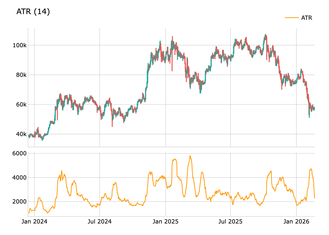

Moving Average Envelope (MAE)

Moving Average Envelopes are percentage-based envelopes set above and below a moving average. The moving average forms the base, and the envelopes are set at a fixed percentage above and below. This indicator is useful for identifying overbought/oversold conditions, spotting trend direction, and finding support and resistance levels.

def movingaverageenvelope(
    data: Union[PdDataFrame, PlDataFrame],
    source_column: str = 'Close',
    period: int = 20,
    percentage: float = 2.5,
    ma_type: str = 'sma',
    middlecolumn: str = 'maenvelope_middle',
    uppercolumn: str = 'maenvelope_upper',
    lowercolumn: str = 'maenvelope_lower'
) -> Union[PdDataFrame, PlDataFrame]:

Example

from investingalgorithmframework import download
from pyindicators import movingaverageenvelope
pl_df = download(     symbol="btc/eur",     market="binance",     time_frame="1d",     start_date="2023-12-01",     end_date="2023-12-25",     save=True,     storage_path="./data" ) pd_df = download(     symbol="btc/eur",     market="binance",     time_frame="1d",     start_date="2023-12-01",     end_date="2023-12-25",     pandas=True,     save=True,     storage_path="./data" )
Calculate Moving Average Envelope for Polars DataFrame
pldf = movingaverageenvelope(pldf, source_column="Close", period=20, percentage=2.5)
pl_df.show(10)
Calculate Moving Average Envelope for Pandas DataFrame
pddf = movingaverageenvelope(pddf, source_column="Close", period=20, percentage=2.5)
pd_df.tail(10)

Nadaraya-Watson Envelope (NWE)

The Nadaraya-Watson Envelope uses Gaussian kernel regression to create a smoothed price estimate, then adds an envelope based on the mean absolute error (MAE) scaled by a multiplier. This is a non-repainting (endpoint) implementation. It is useful for identifying overbought/oversold zones and mean-reversion opportunities.

Calculation:

• Kernel weights: w(i) = exp(-i² / (2 × h²)) for i = 0..lookback-1
• Smoothed value: sum(src[t-i] × w(i)) / sum(w(i))
• MAE: SMA of |src - smoothed| over the lookback period
• Upper: smoothed + mult × MAE
• Lower: smoothed - mult × MAE

def nadarayawatsonenvelope(     data: Union[PdDataFrame, PlDataFrame],     source_column: str = 'Close',     bandwidth: float = 8.0,     mult: float = 3.0,     lookback: int = 500,     uppercolumn: str = 'nweupper',     lowercolumn: str = 'nwelower',     middlecolumn: str = 'nwemiddle', ) -> Union[PdDataFrame, PlDataFrame]:

Example

from investingalgorithmframework import download
from pyindicators import nadarayawatsonenvelope
pl_df = download(     symbol="btc/eur",     market="binance",     time_frame="1d",     start_date="2023-12-01",     end_date="2023-12-25",     save=True,     storage_path="./data" ) pd_df = download(     symbol="btc/eur",     market="binance",     time_frame="1d",     start_date="2023-12-01",     end_date="2023-12-25",     pandas=True,     save=True,     storage_path="./data" )
Calculate Nadaraya-Watson Envelope for Polars DataFrame
pldf = nadarayawatsonenvelope(pldf, source_column="Close", bandwidth=8.0, mult=3.0)
pl_df.show(10)
Calculate Nadaraya-Watson Envelope for Pandas DataFrame
pddf = nadarayawatsonenvelope(pddf, source_column="Close", bandwidth=8.0, mult=3.0)
pd_df.tail(10)

Support and Resistance

Indicators that help identify potential support and resistance levels in the market.

Fibonacci Retracement

Fibonacci retracement levels are horizontal lines that indicate where support and resistance are likely to occur. They are based on Fibonacci numbers and are drawn between a swing high and swing low. The standard levels are 0.0 (0%), 0.236 (23.6%), 0.382 (38.2%), 0.5 (50%), 0.618 (61.8% - Golden Ratio), 0.786 (78.6%), and 1.0 (100%).

The calculation formula is:

Level Price = Swing High - (Swing High - Swing Low) × Fibonacci Ratio

def fibonacci_retracement(
    data: Union[PdDataFrame, PlDataFrame],
    high_column: str = 'High',
    low_column: str = 'Low',
    levels: Optional[List[float]] = None,
    lookback_period: Optional[int] = None,
    swing_high: Optional[float] = None,
    swing_low: Optional[float] = None,
    result_prefix: str = 'fib'
) -> Union[PdDataFrame, PlDataFrame]:

Example

from investingalgorithmframework import download
from pyindicators import fibonacci_retracement
pl_df = download(     symbol="btc/eur",     market="binance",     time_frame="1d",     start_date="2023-12-01",     end_date="2023-12-25",     save=True,     storage_path="./data" ) pd_df = download(     symbol="btc/eur",     market="binance",     time_frame="1d",     start_date="2023-12-01",     end_date="2023-12-25",     pandas=True,     save=True,     storage_path="./data" )
Calculate Fibonacci retracement for Polars DataFrame
pldf = fibonacciretracement(pldf, highcolumn="High", low_column="Low")
pl_df.show(10)
Calculate Fibonacci retracement for Pandas DataFrame
pddf = fibonacciretracement(pddf, highcolumn="High", low_column="Low")
pd_df.tail(10)

Golden Zone

The Golden Zone indicator calculates Fibonacci retracement levels based on the highest high and lowest low over a specified rolling period. The "Golden Zone" refers to the area between the 50% and 61.8% Fibonacci retracement levels, which is often considered a key area for potential price reversals or continuations.

This indicator plots dynamic support/resistance levels that update with each bar, making it useful for identifying potential entry and exit points in trending markets.

The calculation formula is:

Highest High (HH) = Rolling maximum of high prices over length bars Lowest Low (LL) = Rolling minimum of low prices over length bars Diff = HH - LL Upper Level = HH - (Diff × 0.5)      # 50% retracement Lower Level = HH - (Diff × 0.618)    # 61.8% retracement

def golden_zone(
    data: Union[PdDataFrame, PlDataFrame],
    high_column: str = 'High',
    low_column: str = 'Low',
    length: int = 60,
    retracementlevel1: float = 0.5,
    retracementlevel2: float = 0.618,
    uppercolumn: str = 'goldenzone_upper',
    lowercolumn: str = 'goldenzone_lower',
    hhcolumn: str = 'goldenzone_hh',
    llcolumn: str = 'goldenzone_ll'
) -> Union[PdDataFrame, PlDataFrame]:

Example

from investingalgorithmframework import download
from pyindicators import golden_zone
pl_df = download(     symbol="btc/eur",     market="binance",     time_frame="1d",     start_date="2023-12-01",     end_date="2023-12-25",     save=True,     storage_path="./data" ) pd_df = download(     symbol="btc/eur",     market="binance",     time_frame="1d",     start_date="2023-12-01",     end_date="2023-12-25",     pandas=True,     save=True,     storage_path="./data" )
Calculate Golden Zone for Polars DataFrame
pldf = goldenzone(pldf, highcolumn="High", low_column="Low", length=60)
pl_df.show(10)
Calculate Golden Zone for Pandas DataFrame
pddf = goldenzone(pddf, highcolumn="High", low_column="Low", length=60)
pd_df.tail(10)

Golden Zone Signal

The Golden Zone Signal function generates trading signals based on whether the price is within the Golden Zone. It returns a signal value of 1 when the close price is between the upper (50%) and lower (61.8%) boundaries of the Golden Zone, and 0 when the price is outside the zone.

This can be used to identify potential support/resistance areas and generate trading signals when price enters or exits the Golden Zone.

!Important: This function requires the Golden Zone columns to be present in the DataFrame. You must call the goldenzone() function first before using goldenzone_signal().

Signal values:

• 1: Price is within the Golden Zone (potential support/resistance area)
• 0: Price is outside the Golden Zone

def goldenzonesignal(     data: Union[PdDataFrame, PlDataFrame],     close_column: str = 'Close',     uppercolumn: str = 'goldenzone_upper',     lowercolumn: str = 'goldenzone_lower',     signalcolumn: str = 'goldenzone_signal' ) -> Union[PdDataFrame, PlDataFrame]:

Example

from investingalgorithmframework import download
from pyindicators import goldenzone, goldenzone_signal
pl_df = download(     symbol="btc/eur",     market="binance",     time_frame="1d",     start_date="2023-12-01",     end_date="2023-12-25",     save=True,     storage_path="./data" ) pd_df = download(     symbol="btc/eur",     market="binance",     time_frame="1d",     start_date="2023-12-01",     end_date="2023-12-25",     pandas=True,     save=True,     storage_path="./data" )
First calculate Golden Zone, then the signal for Polars DataFrame
pldf = goldenzone(pldf, highcolumn="High", low_column="Low", length=60)
pldf = goldenzonesignal(pldf)
pl_df.show(10)
First calculate Golden Zone, then the signal for Pandas DataFrame
pddf = goldenzone(pddf, highcolumn="High", low_column="Low", length=60)
pddf = goldenzonesignal(pddf)
pd_df.tail(10)

Fair Value Gap (FVG)

A Fair Value Gap (FVG) is a price imbalance that occurs when there's a gap between candlesticks, representing institutional order flow. These gaps often act as support/resistance zones where price tends to return.

Bullish FVG (Gap Up): Occurs when the low of the current candle is higher than the high of the candle 2 bars ago. This creates an upward gap that may act as future support.

Bearish FVG (Gap Down): Occurs when the high of the current candle is lower than the low of the candle 2 bars ago. This creates a downward gap that may act as future resistance.

def fairvaluegap(
    data: Union[PdDataFrame, PlDataFrame],
    high_column: str = 'High',
    low_column: str = 'Low',
    bullishfvgcolumn: str = 'bullish_fvg',
    bearishfvgcolumn: str = 'bearish_fvg',
    bullishfvgtopcolumn: str = 'bullishfvg_top',
    bullishfvgbottomcolumn: str = 'bullishfvg_bottom',
    bearishfvgtopcolumn: str = 'bearishfvg_top',
    bearishfvgbottomcolumn: str = 'bearishfvg_bottom'
) -> Union[PdDataFrame, PlDataFrame]:

Example

import pandas as pd
from pyindicators import fairvaluegap, fvgsignal, fvgfilled
Create sample OHLC data
df = pd.DataFrame({
    'High': [100, 105, 115, 120, 118, 115],
    'Low': [95, 100, 102, 115, 113, 99],
    'Close': [98, 103, 110, 117, 115, 100]
})
Detect Fair Value Gaps
df = fairvaluegap(df)
print(df[['bullishfvg', 'bearishfvg', 'bullishfvgtop', 'bullishfvgbottom']])
Generate signals when price enters an FVG zone
df = fvg_signal(df)
print(df['fvg_signal'])  # 1 = in bullish zone, -1 = in bearish zone, 0 = outside
Detect when FVGs have been filled (mitigated)
df = fvg_filled(df)
print(df[['bullishfvgfilled', 'bearishfvgfilled']])

The fvg_signal function generates signals:

• 1: Price is within a bullish FVG zone (potential long entry)
• -1: Price is within a bearish FVG zone (potential short entry)
• 0: Price is outside any FVG zone

The fvg_filled function detects when FVGs have been mitigated:

• Bullish FVG filled: Price drops to reach the bottom of the gap
• Bearish FVG filled: Price rises to reach the top of the gap

Order Blocks

Order Blocks are zones where institutional traders (banks, hedge funds) placed large orders, causing significant price moves. They represent areas of supply and demand imbalance that often act as support/resistance when price returns.

Bullish Order Block: The last bearish candle before a strong upward move. When price returns to this zone, it often bounces up (support).

Bearish Order Block: The last bullish candle before a strong downward move. When price returns to this zone, it often reverses down (resistance).

Breaker Blocks: When an Order Block is broken (invalidated), it becomes a breaker block and may act as the opposite type of support/resistance.

def order_blocks(
    data: Union[PdDataFrame, PlDataFrame],
    swing_length: int = 10,
    use_body: bool = False,
    high_column: str = 'High',
    low_column: str = 'Low',
    open_column: str = 'Open',
    close_column: str = 'Close',
    bullishobcolumn: str = 'bullish_ob',
    bearishobcolumn: str = 'bearish_ob',
    bullishobtopcolumn: str = 'bullishob_top',
    bullishobbottomcolumn: str = 'bullishob_bottom',
    bearishobtopcolumn: str = 'bearishob_top',
    bearishobbottomcolumn: str = 'bearishob_bottom',
    bullishbreakercolumn: str = 'bullish_breaker',
    bearishbreakercolumn: str = 'bearish_breaker'
) -> Union[PdDataFrame, PlDataFrame]:

Example

import pandas as pd
from pyindicators import orderblocks, obsignal, getactiveorder_blocks
Create sample OHLC data
df = pd.DataFrame({
    'Open': [100, 102, 101, 105, 110, 108, 112, 115, 113, 118],
    'High': [103, 104, 106, 112, 115, 112, 118, 120, 117, 122],
    'Low': [99, 100, 100, 104, 108, 106, 110, 113, 111, 116],
    'Close': [102, 101, 105, 110, 108, 110, 115, 113, 116, 120]
})
Detect Order Blocks
df = orderblocks(df, swinglength=5)
print(df[['bullishob', 'bearishob', 'bullishobtop', 'bullishobbottom']])
Generate signals when price enters an OB zone
df = ob_signal(df)
print(df['ob_signal'])  # 1 = in bullish zone, -1 = in bearish zone, 0 = outside
Get currently active Order Blocks
active = getactiveorderblocks(df, maxbullish=3, max_bearish=3)
print(f"Active bullish OBs: {len(active['bullish'])}")
print(f"Active bearish OBs: {len(active['bearish'])}")

The function returns columns for:

• bullishob / bearishob: 1 when Order Block is detected, 0 otherwise
• bullishobtop / bullishobbottom: Zone boundaries for bullish OBs
• bearishobtop / bearishobbottom: Zone boundaries for bearish OBs
• bullishbreaker / bearishbreaker: 1 when OB is broken (becomes breaker block)

The ob_signal function generates signals:

• 1: Price is within a bullish OB zone (potential long entry)
• -1: Price is within a bearish OB zone (potential short entry)
• 0: Price is outside any OB zone

Breaker Blocks

Breaker Blocks are failed Order Blocks that flip into opposite support/resistance zones after a Market Structure Shift (MSS). Inspired by the "Breaker Blocks with Signals [LuxAlgo]" indicator.

Concept:

• When a bullish MSS occurs (close breaks above the most recent swing high) after a confirmed lower-low pattern, the decisive bullish candle in the up-leg becomes a Bullish Breaker Block (+BB) — acting as future support.
• When a bearish MSS occurs (close breaks below the most recent swing low) after a confirmed higher-high pattern, the decisive bearish candle becomes a Bearish Breaker Block (-BB) — acting as future resistance.

Signals:

• Entry Long (+BB): Price opens between the center line and the top, then closes above the top (bounce confirmation)
• Entry Short (-BB): Price opens between the center line and the bottom, then closes below the bottom
• Cancel: Price closes past the center line without triggering an entry (invalidation)
• Mitigated: Price closes fully through the opposite side of the zone

def breaker_blocks(     data: Union[PdDataFrame, PlDataFrame],     swing_length: int = 5,     use_body: bool = False,     use2candles: bool = False,     stopatfirstcenterbreak: bool = True,     high_column: str = "High",     low_column: str = "Low",     open_column: str = "Open",     close_column: str = "Close", ) -> Union[PdDataFrame, PlDataFrame]:

Returns the following columns:

• bbbullish / bbbearish: 1 when a Breaker Block is formed
• bbtop / bbbottom / bb_center: Active BB zone boundaries (forward-filled)
• bb_direction: 1 for bullish BB, -1 for bearish BB, 0 when no BB is active
• bbentrylong / bbentryshort: 1 when an entry signal fires
• bb_cancel: 1 when the center line is broken (invalidation)
• bb_mitigated: 1 when the BB is fully mitigated

Signal function:

• bb_signal: 1 = long entry, -1 = short entry, 0 = no signal

Example

from investingalgorithmframework import download
from pyindicators import (     breaker_blocks,     breakerblockssignal,     getbreakerblocks_stats, )
pd_df = download(     symbol="btc/eur",     market="bitvavo",     time_frame="4h",     start_date="2024-01-01",     end_date="2024-06-01",     pandas=True, )
Detect Breaker Blocks
pddf = breakerblocks(pddf, swinglength=5)
pddf = breakerblockssignal(pddf)
Get summary statistics
stats = getbreakerblocksstats(pddf)
print(stats)
pddf[["Close", "bbbullish", "bbbearish", "bbtop", "bb_bottom",        "bbentrylong", "bbentryshort", "bb_signal"]].tail(10)

Mitigation Blocks

Mitigation Blocks identify the first candle that initiates an impulsive move leading to a Market Structure Shift — the origin of institutional order flow.

Concept (ICT / Smart Money):

• While an Order Block is the last opposing candle before an impulse, a Mitigation Block is the first same-direction candle that starts the move.
• Bullish Mitigation Block: After a bullish MSS (close breaks swing high with confirmed LL pattern), the first bullish candle (close > open) after the preceding swing low that kicked off the upward impulse.
• Bearish Mitigation Block: After a bearish MSS (close breaks swing low with confirmed HH pattern), the first bearish candle (close < open) after the preceding swing high that kicked off the downward impulse.
• When price returns to a Mitigation Block zone, institutional traders are "mitigating" (closing/adjusting) positions opened at that origin candle.

Signals:

• Entry Long: Price retraces into the bullish MB zone (potential long entry)
• Entry Short: Price retraces into the bearish MB zone (potential short entry)
• Mitigated: Price closes through the opposite side of the zone (block invalidated)

def mitigation_blocks(     data: Union[PdDataFrame, PlDataFrame],     swing_length: int = 5,     use_body: bool = False,     high_column: str = "High",     low_column: str = "Low",     open_column: str = "Open",     close_column: str = "Close", ) -> Union[PdDataFrame, PlDataFrame]:

Returns the following columns:

• mbbullish / mbbearish: 1 when a Mitigation Block is established
• mbtop / mbbottom: Active MB zone boundaries (forward-filled)
• mb_direction: 1 for bullish MB, -1 for bearish MB, 0 when no MB is active
• mbentrylong / mbentryshort: 1 when price enters the MB zone
• mb_mitigated: 1 when the MB zone is mitigated

Signal function:

• mb_signal: 1 = long entry, -1 = short entry, 0 = no signal

Example

from investingalgorithmframework import download
from pyindicators import (     mitigation_blocks,     mitigationblockssignal,     getmitigationblocks_stats, )
pd_df = download(     symbol="btc/eur",     market="bitvavo",     time_frame="4h",     start_date="2024-01-01",     end_date="2024-06-01",     pandas=True, )
Detect Mitigation Blocks
pddf = mitigationblocks(pddf, swinglength=5)
pddf = mitigationblockssignal(pddf)
Get summary statistics
stats = getmitigationblocksstats(pddf)
print(stats)
pddf[["Close", "mbbullish", "mbbearish", "mbtop",        "mbbottom", "mbentrylong", "mbentry_short",        "mb_signal"]].tail(10)

Rejection Blocks

Rejection Blocks identify candles at swing extremes whose disproportionately long wicks signal institutional rejection of a price level, creating a tradeable zone.

Concept (ICT / Smart Money):

• A Rejection Block forms when a candle at a pivot point has a wick that is at least wick_threshold (default 50 %) of the total candle range.
• The long wick shows that price was driven to a level but was rejected — institutional participants absorbed the orders and pushed price back.
• Bullish Rejection Block: At a confirmed swing low, the candle's lower wick (Low → body bottom) is disproportionately large. The zone spans the lower wick area.
• Bearish Rejection Block: At a confirmed swing high, the candle's upper wick (body top → High) is disproportionately large. The zone spans the upper wick area.
• When price returns to this wick zone, the same institutional interest is expected — a potential trade entry.

Signals:

• Entry Long: Price retraces into the bullish RB zone (potential long entry)
• Entry Short: Price retraces into the bearish RB zone (potential short entry)
• Mitigated: Price closes through the opposite side of the zone (block invalidated)

def rejection_blocks(     data: Union[PdDataFrame, PlDataFrame],     swing_length: int = 5,     wick_threshold: float = 0.5,     high_column: str = "High",     low_column: str = "Low",     open_column: str = "Open",     close_column: str = "Close", ) -> Union[PdDataFrame, PlDataFrame]:

Returns the following columns:

• rbbullish / rbbearish: 1 when a Rejection Block is established
• rbtop / rbbottom: Active RB zone boundaries (forward-filled)
• rb_direction: 1 for bullish RB, -1 for bearish RB, 0 when no RB is active
• rbentrylong / rbentryshort: 1 when price enters the RB zone
• rb_mitigated: 1 when the RB zone is mitigated

Signal function:

• rb_signal: 1 = long entry, -1 = short entry, 0 = no signal

Example

from investingalgorithmframework import download
from pyindicators import (     rejection_blocks,     rejectionblockssignal,     getrejectionblocks_stats, )
pd_df = download(     symbol="btc/eur",     market="bitvavo",     time_frame="4h",     start_date="2024-01-01",     end_date="2024-06-01",     pandas=True, )
Detect Rejection Blocks
pddf = rejectionblocks(pddf, swinglength=5, wick_threshold=0.5)
pddf = rejectionblockssignal(pddf)
Get summary statistics
stats = getrejectionblocksstats(pddf)
print(stats)
pddf[["Close", "rbbullish", "rbbearish", "rbtop",        "rbbottom", "rbentrylong", "rbentry_short",        "rb_signal"]].tail(10)

Optimal Trade Entry (OTE)

Identifies ICT Optimal Trade Entry zones — the Fibonacci 61.8 %–78.6 % retracement of an impulse leg following a Market Structure Shift (MSS).

Concept (ICT / Smart Money):

• After a Break of Structure, the market typically retraces before continuing. The OTE zone (61.8 %–78.6 % Fibonacci retracement) is where institutional traders are most likely to enter or add to positions.
• Bullish OTE: After a bullish MSS (close breaks swing high with confirmed Lower Low), the OTE zone is the 61.8 %–78.6 % pullback of the impulse leg from swing low to the MSS bar.
• Bearish OTE: After a bearish MSS (close breaks swing low with confirmed Higher High), the OTE zone is the 61.8 %–78.6 % retracement from swing high down to the MSS bar.

Signals:

• Entry Long: Price retraces into the bullish OTE zone (potential long entry)
• Entry Short: Price retraces into the bearish OTE zone (potential short entry)
• Invalidated: Price closes beyond the impulse origin (zone no longer valid)

Optional Premium/Discount filter: Only emit bullish OTEs when the impulse origin is in the discount zone, and bearish OTEs when in the premium zone.

```python def optimal_t

---

README truncated. View on GitHub