TSstudio

The TSstudio package provides a set of tools descriptive and predictive analysis of time series data. That includes utility functions for preprocessing time series data, interactive visualization functions based on the plotly package engine, and set of tools for training and evaluating time series forecasting models from the forecast, forecastHybrid, and bsts packages.

More information available on the package vignettes.

Installation

Install the stable version from CRAN:

r
install.packages("TSstudio")

or install the development version from Github:

r
install.packages("devtools")
devtools::install_github("RamiKrispin/TSstudio")

Usage

Plotting time series data

r
library(TSstudio)
data(USgas)
Ploting time series object
ts_plot(USgas, 
        title = "US Monthly Natural Gas Consumption",
        Ytitle = "Billion Cubic Feet")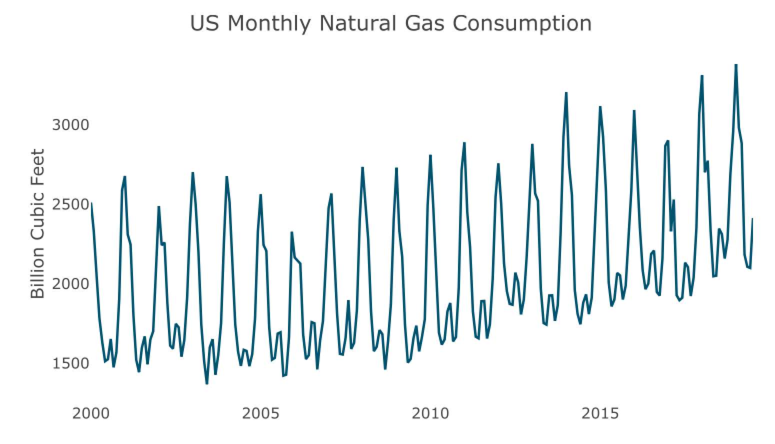

Seasonality analysis

r
Seasonal plot
ts_seasonal(USgas, type = "all")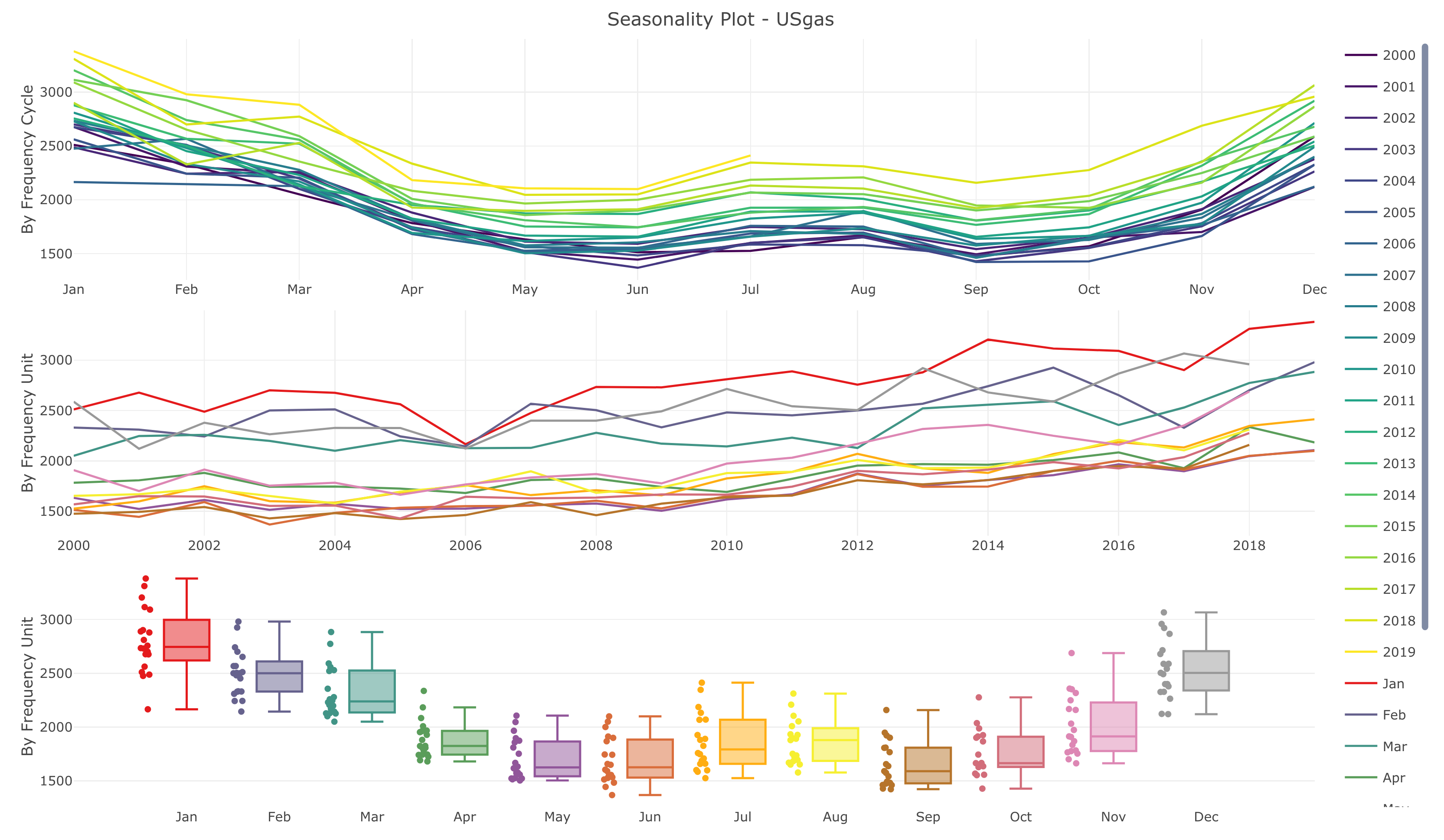

r
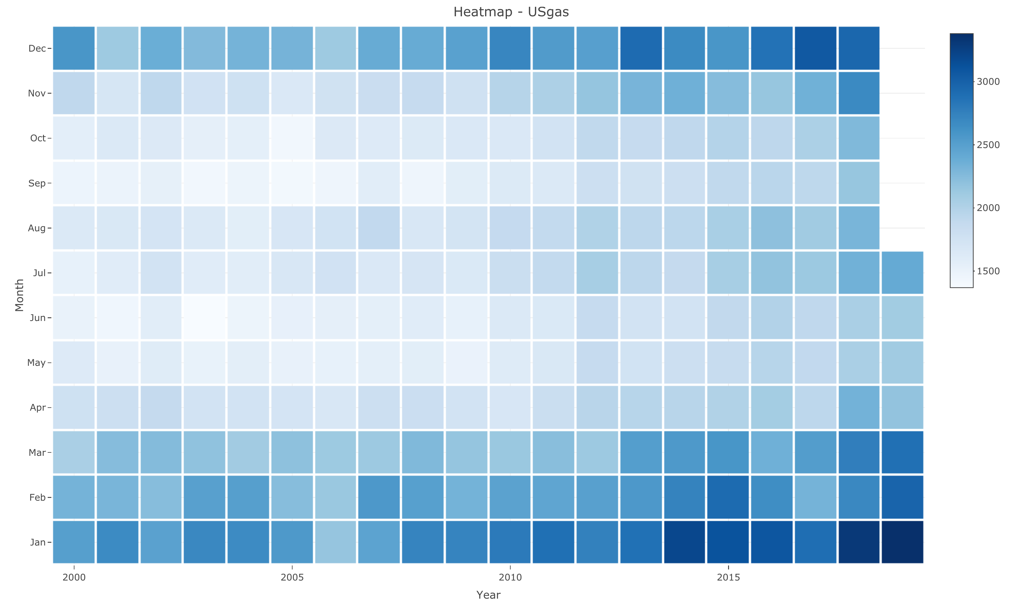
Heatmap plot
ts_heatmap(USgas)

Correlation analysis

r
ACF and PACF plots
ts_cor(USgas, lag.max = 60)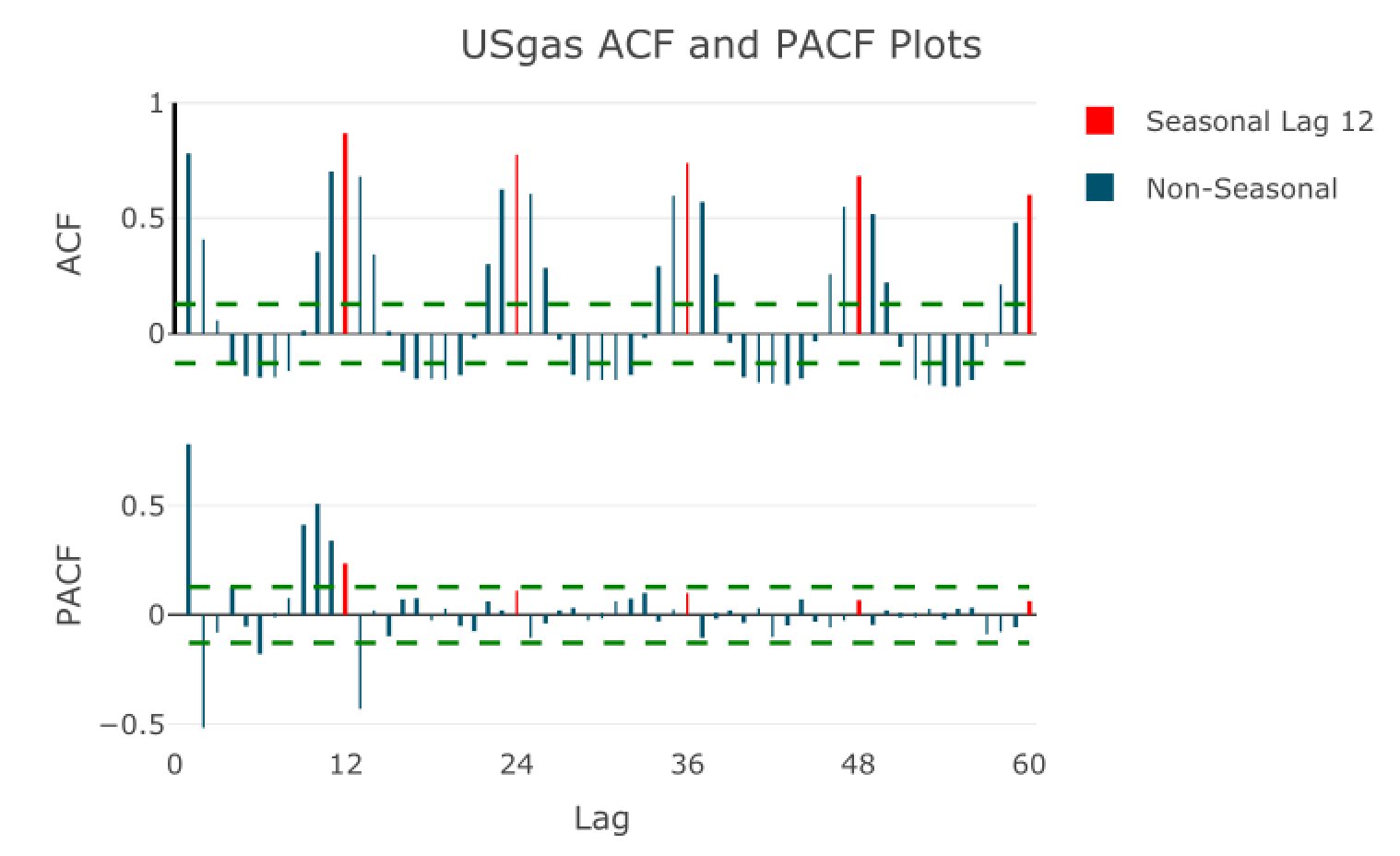

r
Lags plot
ts_lags(USgas, lags = 1:12)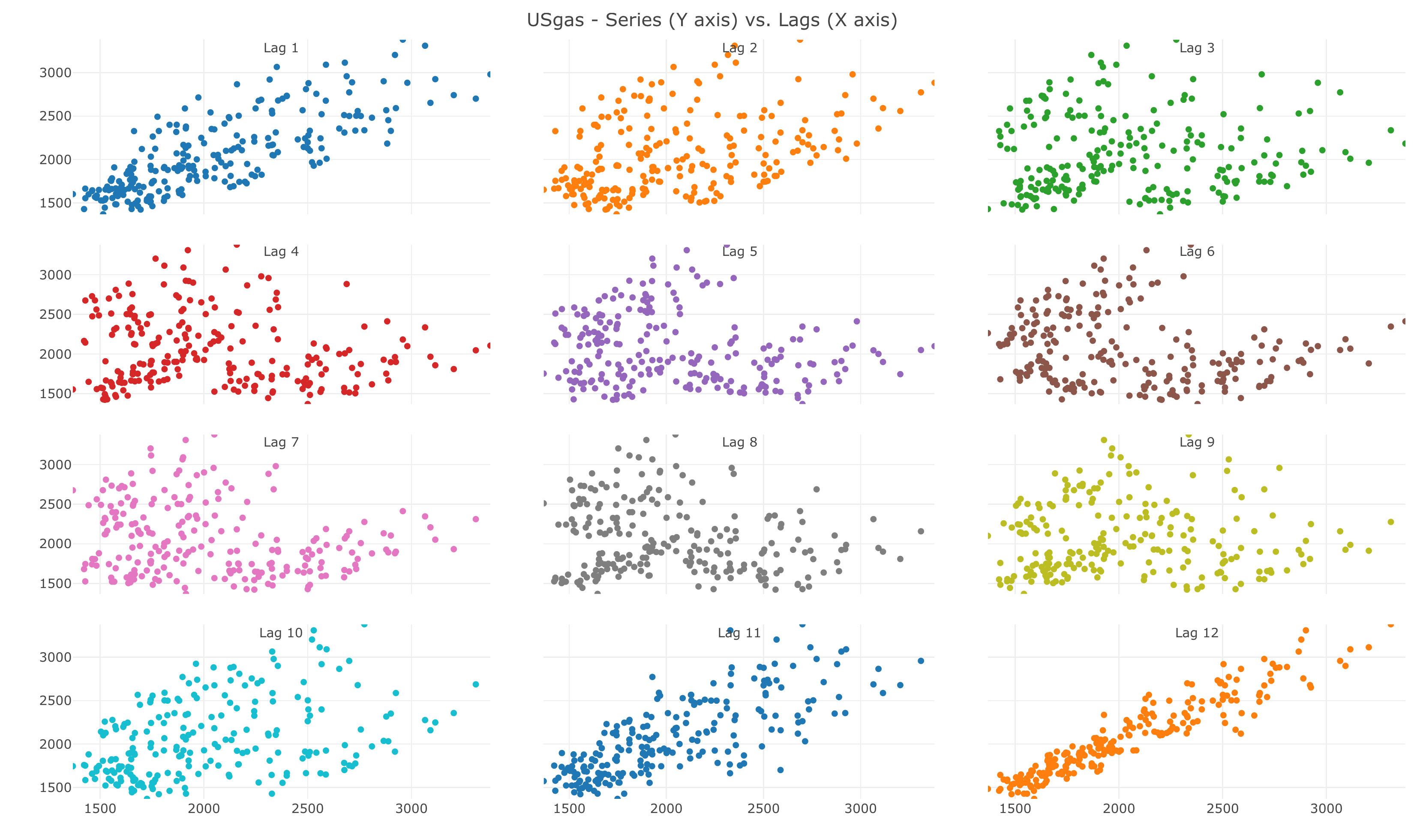

r
Seasonal lags plot
ts_lags(USgas, lags = c(12, 24, 36, 48))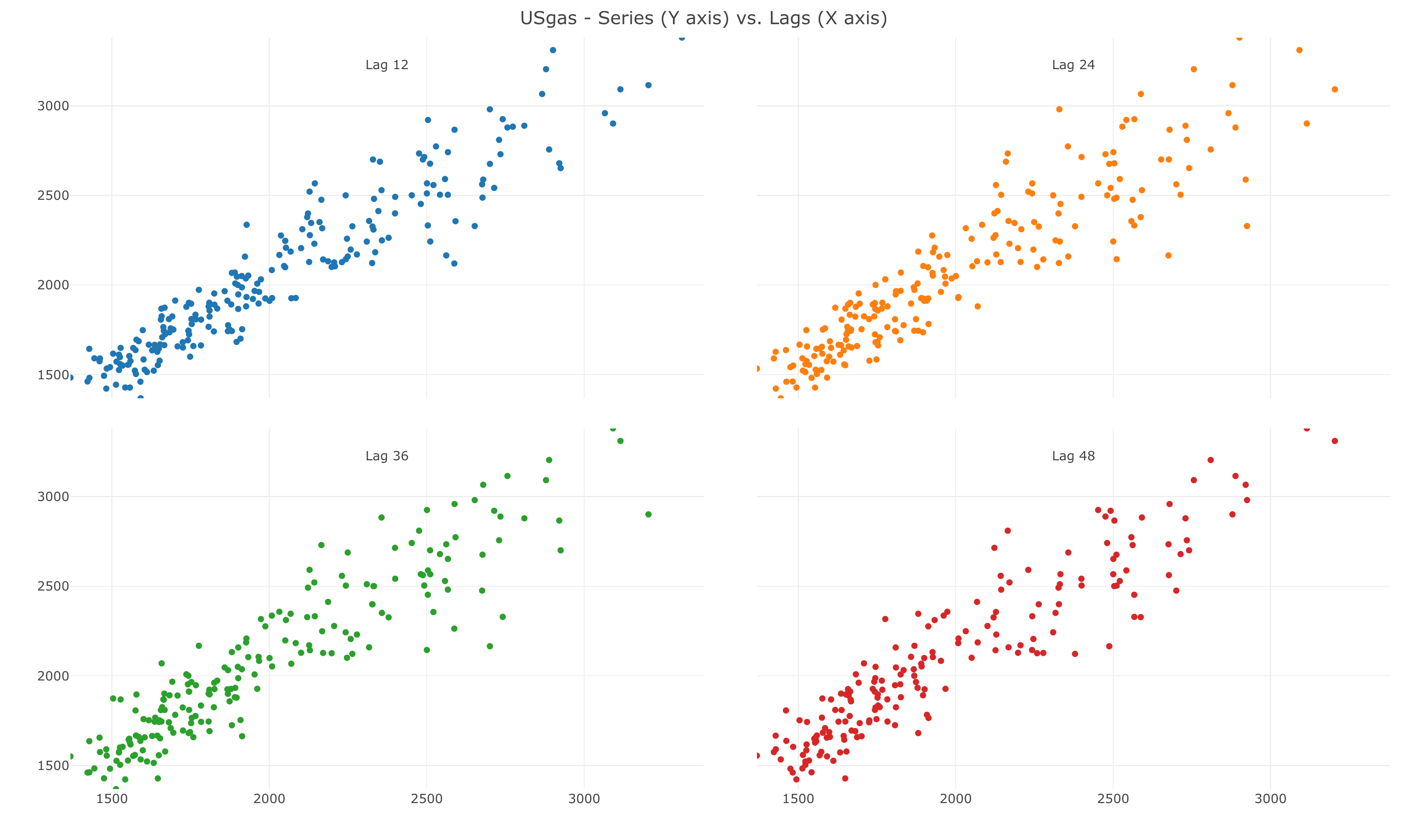

Training forecasting models

r
Forecasting applications
Setting training and testing partitions
USgass <- tssplit(ts.obj = USgas, sample.out = 12)
train <- USgas_s$train
test <- USgas_s$test
Forecasting with auto.arima
library(forecast)
md <- auto.arima(train)
fc <- forecast(md, h = 12)
Plotting actual vs. fitted and forecasted
test_forecast(actual = USgas, forecast.obj = fc, test = test)

r
Plotting the forecast 
plot_forecast(fc)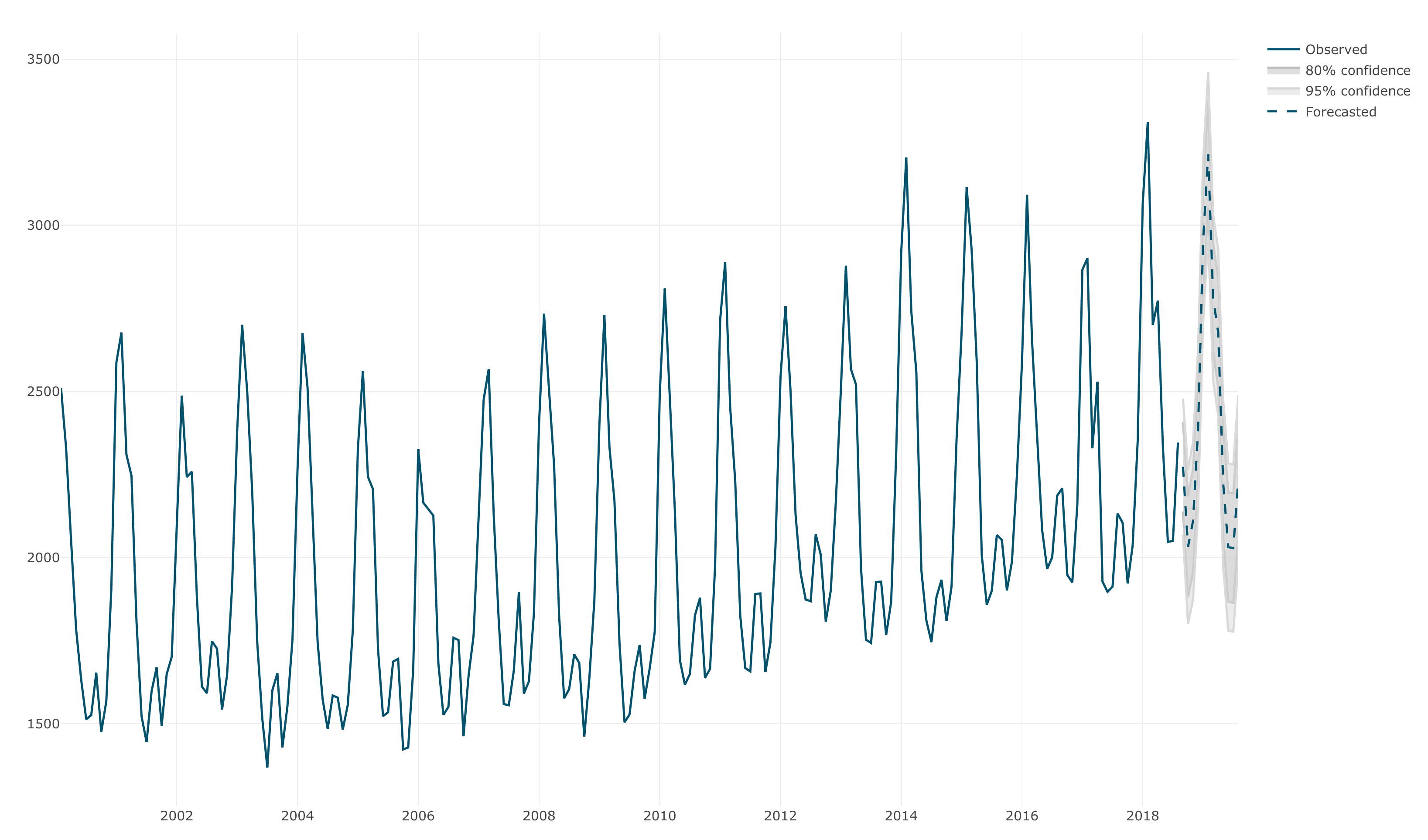

r
Run horse race between multiple models
methods <- list(ets1 = list(method = "ets",
                            method_arg = list(opt.crit = "lik"),
                            notes = "ETS model with opt.crit = lik"),
                ets2 = list(method = "ets",
                            method_arg = list(opt.crit = "amse"),
                            notes = "ETS model with opt.crit = amse"),
                arima1 = list(method = "arima",
                              method_arg = list(order = c(2,1,0)),
                              notes = "ARIMA(2,1,0)"),
                arima2 = list(method = "arima",
                              method_arg = list(order = c(2,1,2),
                                                seasonal = list(order = c(1,1,1))),
                              notes = "SARIMA(2,1,2)(1,1,1)"),
                hw = list(method = "HoltWinters",
                          method_arg = NULL,
                          notes = "HoltWinters Model"),
                tslm = list(method = "tslm",
                            method_arg = list(formula = input ~ trend + season),
                            notes = "tslm model with trend and seasonal components"))
Training the models with backtesting
md <- train_model(input = USgas,
                  methods = methods,
                  train_method = list(partitions = 6, 
                                      sample.out = 12, 
                                      space = 3),
                  horizon = 12,
                  error = "MAPE")
A tibble: 6 x 7
  modelid model       notes                                         avgmape avgrmse avgcoverage80% avgcoverage_95%
  <chr>    <chr>       <chr>                                            <dbl>    <dbl>              <dbl>              <dbl>
1 arima2   arima       SARIMA(2,1,2)(1,1,1)                            0.0557     167.              0.583              0.806
2 hw       HoltWinters HoltWinters Model                               0.0563     163.              0.736              0.889
3 ets1     ets         ETS model with opt.crit = lik                   0.0611     172.              0.681              0.903
4 ets2     ets         ETS model with opt.crit = amse                  0.0666     186.              0.458              0.833
5 tslm     tslm        tslm model with trend and seasonal components   0.0767     220.              0.417              0.667
6 arima1   arima       ARIMA(2,1,0)                                    0.188      598.              0.875              0.958

r
Plot the performance of the different models on the testing partitions
plot_model(md)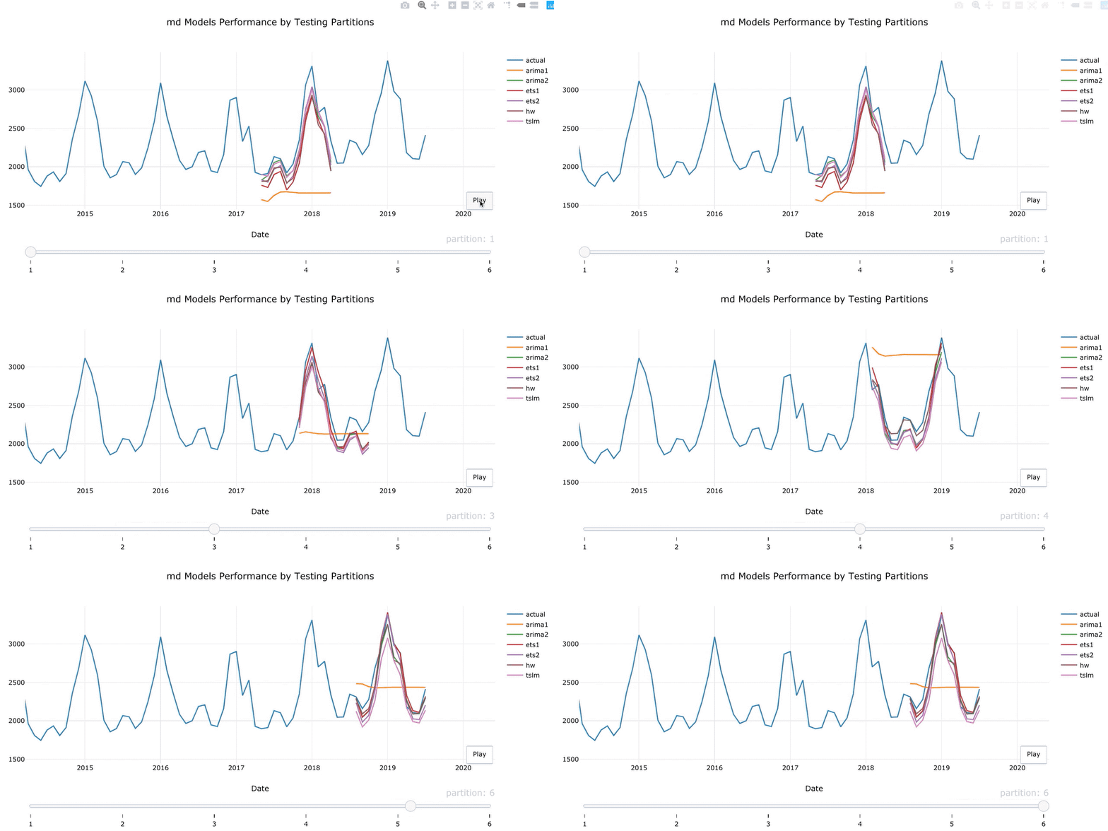

r
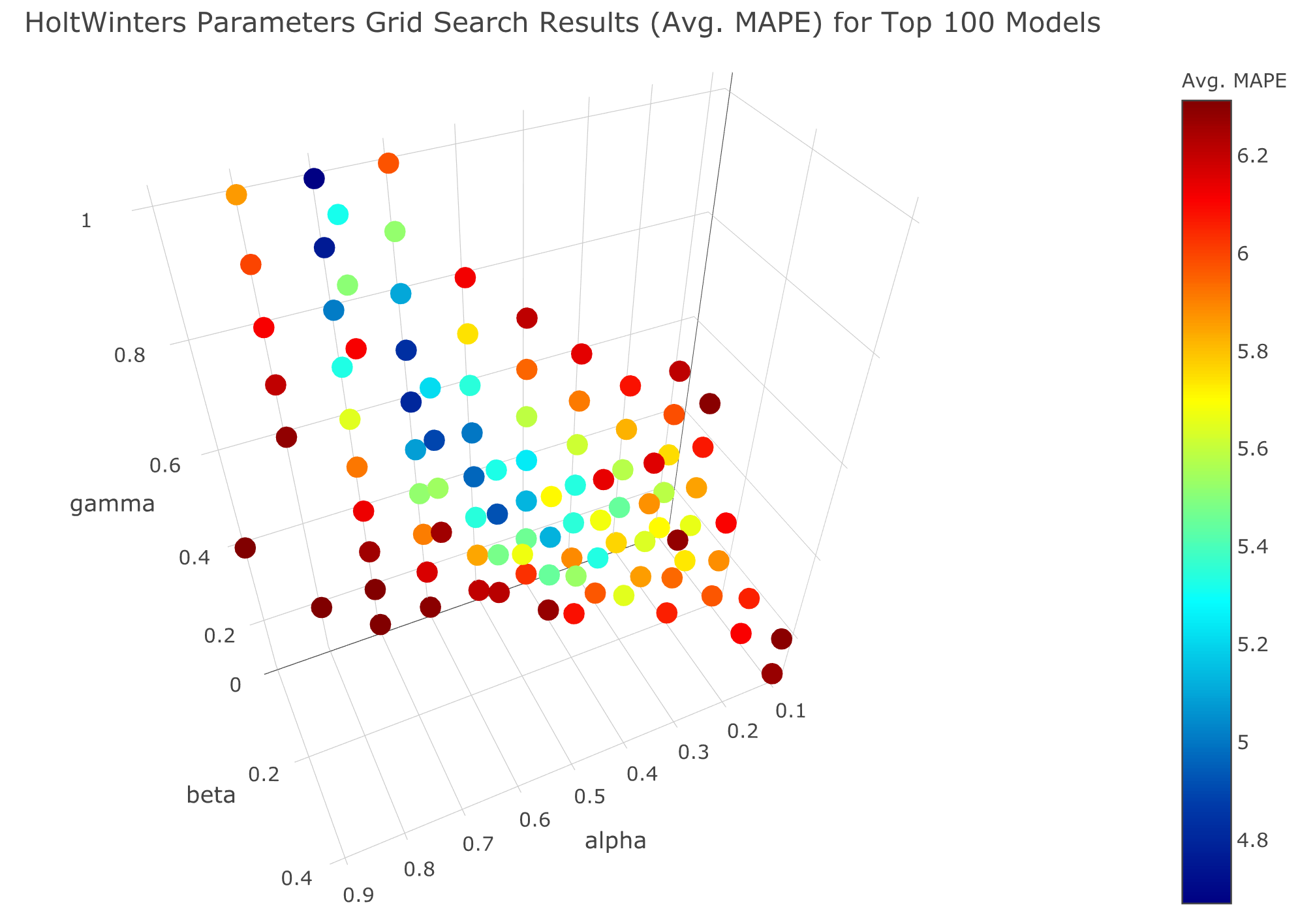
Holt-Winters tunning parameters with grid search
hwgrid <- tsgrid(USgas, 
                   model = "HoltWinters",
                   periods = 6,
                   window_space = 6,
                   window_test = 12,
                   hyper_params = list(alpha = seq(0,1,0.1),
                                       beta = seq(0,1,0.1),
                                       gamma = seq(0,1,0.1)))
                                       
plotgrid(hwgrid, type = "3D")

🔗 More in this category