No description available.

Data Engineering Capstone Project for Udacity
Objective
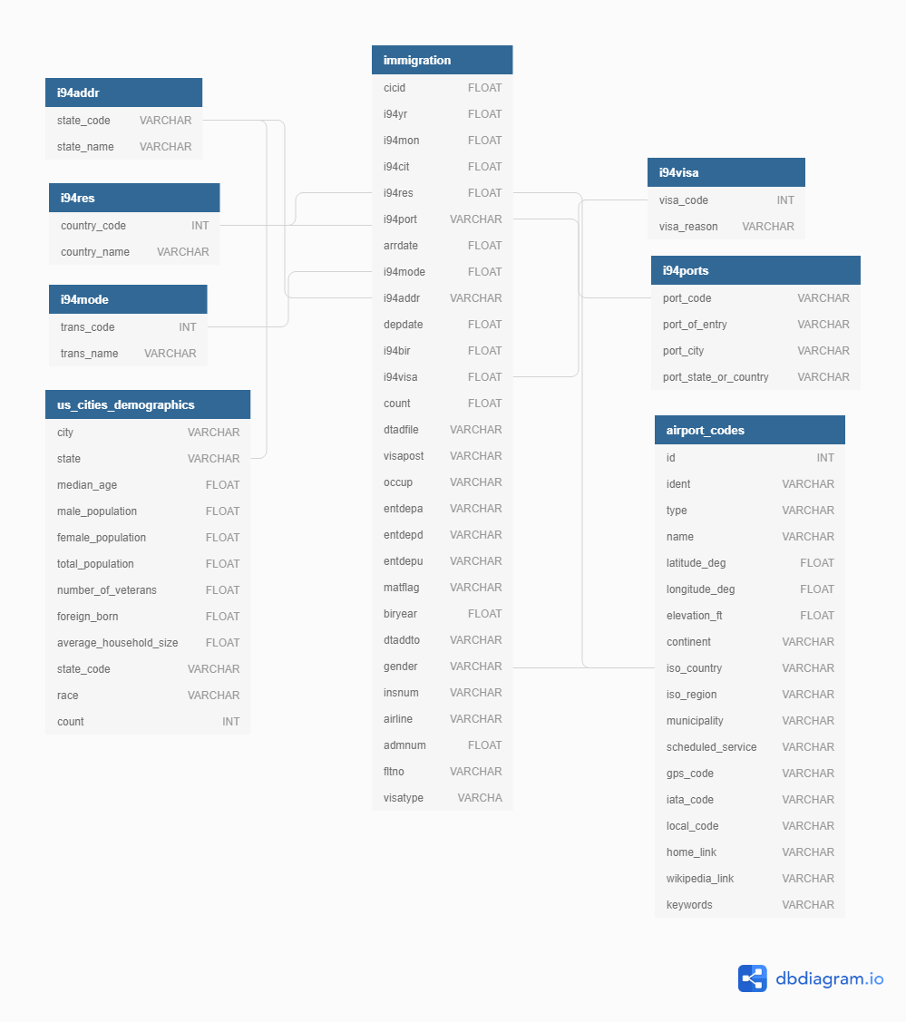
In this project we are going to work with US immigraton data from the year 1994. We have facts such as visa types, transport modes, landing ports, us state codes, country codes. Apart from the sas7bdat formatted immigration data we have us airport information and us demographics data. We are going to parse SAS descriptor files for all the dimensions and sas7bdat files for all the facts. The tools we are going to use here are Apache Spark, Apache Airflow, Amazon Redshift, Amazon S3.
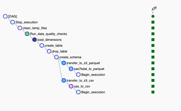
We will be reading, parsing and cleaning the data from local file systems, Amazon S3 and transferring data to redshift tables in AWS. We will be orchestrating the flow of data through Apache Airflow DAGs.
Finally we will be using some SQL queries to extract some valuable stats and graphs from the data itself.
Data Model
Data Pipeline


Installing and starting
Installing Python Dependencies
You need to install this python dependencies In Terminal/CommandPrompt:without anaconda you can do this:
$ python3 -m venv virtual-env-name $ source virtual-env-name/bin/activate $ pip install -r requirements.txt$ conda env create -f env.yml $ source activate <conda-env-name>conda create -y -n <conda-env-name> python==3.6 conda install -f -y -q -n <conda-env-name> -c conda-forge --file requirements.txt [source activate/ conda activate] <conda-env-name>Fixing/Configuring Airflow
$ pip install --upgrade Flask $ pip install zappa $ mkdir airflow_home $ export AIRFLOWHOME=./airflowhome $ cd airflow_home $ airflow initdb $ airflow webserver $ airflow schedulerMore Airflow commands
To list existing dags registered with airflow$ airflow list_dagsSecure/Encrypt your connections and hooks
Run$ python cryptosetup.pySetting up connections and variables in Airflow UI for AWS
TODO: There is no code to modify in this exercise. We're going to create a connection and a variable.S3
- Open your browser to localhost:8080 and open Admin->Variables
- Click "Create"
- Set "Key" equal to "s3_bucket" and set "Val" equal to "udacity-dend"
- Set "Key" equal to "s3_prefix" and set "Val" equal to "data-pipelines"
- Click save
- Open Admin->Connections
- Click "Create"
- Set "Conn Id" to "aws_credentials", "Conn Type" to "Amazon Web Services"
- Set "Login" to your awsaccesskeyid and "Password" to your awssecret_key
- Click save
- If it doesn't work then in "Extra" field put:
- These are all you can put:
- awsaccountid: AWS account ID for the connection
- awsiamrole: AWS IAM role for the connection
- external_id: AWS external ID for the connection
- host: Endpoint URL for the connection
- region_name: AWS region for the connection
- role_arn: AWS role ARN for the connection
- Open Admin->Connections
- Click "Create"
- Set "Conn Id" to "redshift", "Conn Type" to "postgres"
- Set "Login" to your master_username for your cluster and "Password"
- Click save
Optional
If you haven't setup your AWS Redshift Cluster yet (or don't want to create one manually), then use the files inside 'aws' folder- To create cluster and IAM role: Run the below code in terminal from 'aws' folder to create your Redshift database and a
$ python aws_operate.py --action start- To create Tables: Run the below code in terminal from project dir to create tables in your Redshift database
$ python createtable.py --host <clusterendpoint_address>
- To Stop: Run the below code in terminal from 'aws' directory to destroy your Redshift database and
detach iam_role from the cluster### About the data
I94 Immigration Data:
This data comes from the US National Tourism and Trade Office.
This
is where the data comes from. There's a sample file so you can take a look
at the data in csv format before sreading it all in. The report contains
international visitor arrival statistics by world regions and selected
countries (including top 20), type of visa, mode of transportation,
age groups, states visited (first intended address only), and the top
ports of entry (for select countries)
World Temperature Data:
This dataset came from Kaggle. You can read more about it here.
U.S. City Demographic Data:
This data comes from OpenSoft. You can read more about it here.
Airport Code Table:
This is a simple table of airport codes and corresponding cities. It comes from here.
Run the project
- Follow all the setup mentioned above
- Create a bucket in region 'us-west-2' in Amazon S3
- You have to setup all the connections and variables in the Airflow
admin
i. Setup aws connection with user credentials (access_key and
secret_key with login and password). Make sure the region is 'us-west-2'
ii. Setup Redshift connection with user, password, host, port,
schema, db
iii. Setup iam_role for your aws account
iv. Setup variables for 'tempinput', 'tempoutput', 'spark_path' (spark
manipulation path for parquet files), sas_file (sas7bdat descriptor
files)
v. Place all the csv inputs inside temp_output directory
vi. Create a folder called 'spark_path' inside \airflow\dags\
vii. Create variable called 's3_bucket' (make sure the bucket in
AWS is in region 'us-west-2')
Example:
| variable | example value |
|:-------------|-------------:|
| iam_role | #### |
| s3_bucket | #### |
| sasfile | /home/workspace/airflow/dags/tempinput/I94SASLabels_Descriptions.SAS |
| sparkpath | /home/workspace/airflow/dags/sparkpath |
| tempinput | /home/workspace/airflow/dags/tempinput/ |
| tempoutput | /home/workspace/airflow/dags/tempoutput/ |
- Data Location for input files:
i. Put all your sas7bdat formatted files in temp_input directory
(whenever you want to process/insert them into the db, when you are
done remove the .sas7bdat file/files and drop new files)
ii. Put SAS descriptor file in temp_input directory
iii. Put airport-codescsv.csv file in tempoutput directory
Test it Yourself!
Here are some example queries we test to see the uploaded results into the Redshift schema Example Queries
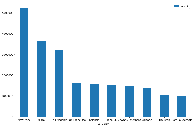
City from where immigrants arrived
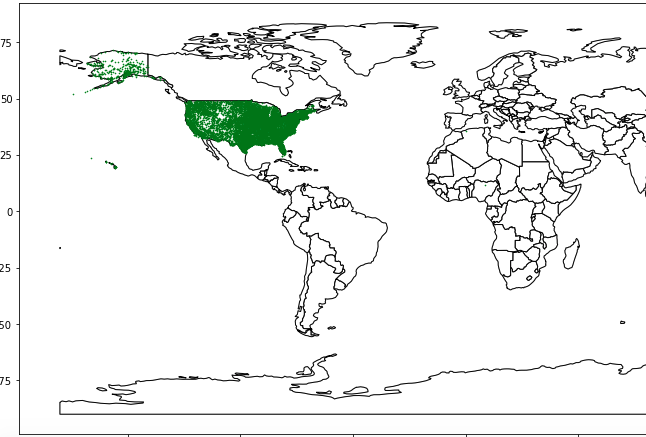
#### Different kinds of airports#### Immigrants from different countries#### Small airports from different states#### Small airport locations### Stats and Graphs
City from where immigrants arrived
Different kinds of airports

Immigrants from different countries

Small airports from different states

Small airports locations in different states
Scoping the Project
The purpose is to produce interesting stats from the US immigration data, airports around the world, and different dimensions such as visa type, transport mode, nationality etc.
Steps Taken:
The steps taken are in the following order:
Gather the data:
This took a while as different kinds of formats were chosen, I
needed to fix my mindset on which data I will actually use in
future for my analysis and queries. I fixated on .sas7bdat
formatted immigration data which fulfills the minimum number of
rows requirements, the cleaned airport data for dimensions and
SAS descriptor file for fulfilling the different kind of formats
to be chosen for the project
Study the data:
This took a while as I needed to understand what kind of
pre-processing I would use to clean the individual datasets
mentioned above. Dropping rows on a condition, filtering rows
according to other dimensions and facts etc.
Choice of infrastructure:
After studying the data I decided upon certain tools and
technologies, to the point where I am comfortable; I made use of
maximum number of skills that I think I learnt through out the
process.
Implementation and Testing:
Once my pipeline started running, I did all kinds of quality
checks to ensure that data is processed correctly and provided a
Jupyter notebook to test the project.
Purpose of Final Data Model:
Gather interesting insights like demographic population based on certain
dimensions based upon some filter conditions.
e.g.
- Compare immigration of different nationalities
- Compare number of airports by state
- Different kinds of airport statistics
- Aggregate flow of immigrants through different cities
So I am using the airport codes, US immigration data of '94 and dimensions such as visa type, mode of transport, nationality codes, US state code information
Addressing other scenarios
Data Increased by 100x:
- I am using columnar format of redshift, so querying will not be slower
- Incremental update is provided so that every time full amount is not
inserted everytime. Whenever one wants to insert data into the database
for immigration can just drop their sas7bdat files into the temp_input
folder
- Spark is used where heavy data is read and parsed, so distributed
processing is also involved
- Spark memory and processors is configurable to handle more pressure
- S3 storage is used which is scalable and easily accessible with other
AWS infrastructure
The pipelines would be run on a daily basis by 7 am every day:
- The pipeline is scheduled as per requirements
The database needed to be accessed by 100+ people:
- People are granted usage on schema, so not everyone but people who
have access to the data can use it as necessary, below are the
necessary commands one you use in Redshift query editor, that's why it
is purely optional to use it as a task in the pipeline:
We can create a group of users, called webappusers, who will use the use the functionality of the schema but cannot take admin decisions and we can add individual users with their name and init password.
We can create a group of users called webdevusers, who will have admin privileges on the schema, we can add those individual users with their name and init passwordDefending Decisions
The choice of tools, technologies:
- Airflow to view, monitor and log flow of information: Extremely useful tool to control end to end ETL processing
- S3 Storage to store data on a large scale: Never complain about storage and most importantly when it stores big data
- Redshift to make advantage of columnar format and faster querying strategies: Query from anywhere and anytime
- Spark for distributed processing of heavy data: Best in-memory faster processing
- Pandas for cleaning data frames: absolutely neccessary
Links for Airflow
Context Variables https://airflow.apache.org/macros.html
Hacks for airflow https://medium.com/datareply/airflow-lesser-known-tips-tricks-and-best-practises-cf4d4a90f8f https://medium.com/handy-tech/airflow-tips-tricks-and-pitfalls-9ba53fba14eb https://www.astronomer.io/guides/dag-best-practices/
Technologies Used