Topological Data Analysis of Market Crashes

A reproduction and out-of-sample extension of Gidea and Katz (2017), *Topological Data Analysis of Financial Time Series: Landscapes of Crashes* (arXiv:1703.04385), run on four US equity indices from 1992 to 2026.

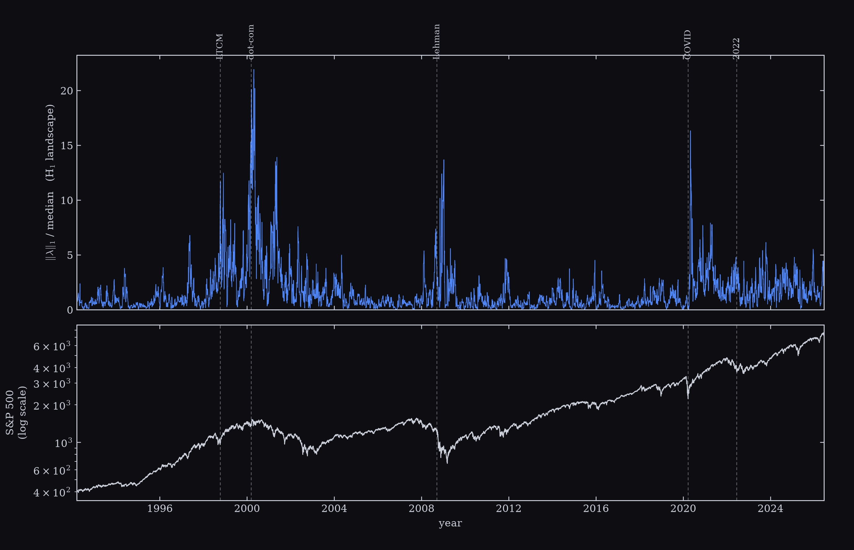
The headline result is a single number per day that spikes at every crash. The point of the project is to ask what that number actually measures, and whether it can predict anything. The honest answers are: it measures decoupling, not volatility or crash size, and no, it does not forecast crashes. It describes, precisely and after the fact, how a market came apart.

Method in a paragraph

Take four US indices (S&P 500, Dow Jones, NASDAQ, Russell 2000). Each trading day, the four daily log returns form a single point in R^4. A sliding window of 50 trading days is therefore a cloud of 50 points. We build the Vietoris-Rips filtration on that cloud and compute its persistent homology with ripser; the first homology H1 counts loops. Each window's H1 diagram is summarized by the L^p norms of its Bubenik persistence landscape, with the L^1 norm given in closed form by the sum of (death - birth)^2 / 4 over the diagram. That is one number per day. Plotted over 34 years, it spikes at every crash.

Key findings

• It measures decoupling, not magnitude. The largest spike in the whole record is the dot-com

crash, not COVID, even though COVID ran roughly three times the realized volatility (peak about 98% versus 36% annualized). In 2000 the indices came apart (mean pairwise correlation 0.63, with the NASDAQ pulling away from the rest); in March 2020 they fell together (0.97). The norm tracks whether the market moves as one thing or many, not how far it falls.

• As a forecaster it is weak, and we say so. The norm level lags: on the day the market

bottomed in COVID it was still at its baseline median. The variance of the norm builds before slow, endogenous crashes (the dot-com run-up shows a real rise over the year, Mann-Kendall tau = +0.33) but stays flat before an exogenous shock (COVID) and only explodes at the crash itself. So the warning lead collapses: about a year before the dot-com top, a few months before Lehman, nothing before COVID. Out of sample, for a worst-decile forward 20-day drawdown, the topological norm scores AUC 0.62, below plain realized volatility at 0.66, and a variance alarm fires with only about 1.18x lift over the base rate.

Repository layout

marketcrashtda.ipynb   the full write-up: theory, worked example, reproduction, statistics. Start here.
scripts/                 the analysis code
data/                    price series (Yahoo) and precomputed landscape norms
figures/                 generated figures

Install

python -m venv .venv
Windows:  .venv\Scripts\activate     macOS/Linux:  source .venv/bin/activate
pip install -r requirements.txt

Reproduce

The notebook runs the whole story end to end and is the recommended entry point:

jupyter notebook marketcrashtda.ipynb

The individual figures are produced by the scripts. Run them from the repository root (paths are resolved relative to it):

| command | output | |---|---| | python scripts/crashlandscape.py | figures/crashlandscape.png (Gidea-Katz Fig. 9, 1998-2010; also writes data/landscape_norms.csv) | | python scripts/fullhistory.py | figures/fullhistory.png (norm and S&P, 1992-2026) | | python scripts/recent.py | figures/recent_landscape.png (2017-2026, out of sample) | | python scripts/decompose.py | figures/decompose.png (norm vs realized vol vs mean correlation) | | python scripts/diagnosticsplots.py | figures/decouplingmap.png, adaptivez.png, leadmultiples.png | | python scripts/ewsvariance.py | figures/ewsvariability.png (norm variability into each crash) | | python scripts/ewsvalidate.py | figures/ewspeak.png and the AUC / alarm statistics | | python scripts/leadtime.py | figures/leadtime.png | | python scripts/statisticsreport.py | figures/rocprediction.png and the inferential statistics | | python scripts/aucdiff.py / leadlag.py / full_analysis.py | console statistics only |

Data

Prices are fetched from the public Yahoo Finance chart API by the scripts. The CSVs are committed so the repository runs without a network call, which also pins the exact series used. The landscape norms (data/norms.csv, data/landscape_norms.csv) are computed by the scripts and committed as a cache; delete them to recompute from scratch (this takes a while, since it runs ripser over thousands of windows).

Citation

If you use this, please cite the original paper. It is not redistributed here:

Gidea, M., and Katz, Y. (2017). Topological Data Analysis of Financial Time Series: Landscapes of

Crashes. Physica A: Statistical Mechanics and its Applications. arXiv:1703.04385.

License

MIT, see LICENSE.