
After watching all the videos of the famous Standford's CS231n course that took place in 2017, i decided to take summary of the whole course to help me to remember and to anyone who would like to know about it. I've skipped some contents in some lectures as it wasn't important to me.
Standford CS231n 2017 Summary
After watching all the videos of the famous Standford's CS231n course that took place in 2017, i decided to take summary of the whole course to help me to remember and to anyone who would like to know about it. I've skipped some contents in some lectures as it wasn't important to me.
Table of contents
* Table of contents * Course Info * 01. Introduction to CNN for visual recognition * 02. Image classification * 03. Loss function and optimization * 04. Introduction to Neural network * 05. Convolutional neural networks (CNNs) * 06. Training neural networks I * 07. Training neural networks II * 08. Deep learning software * 09. CNN architectures * 10. Recurrent Neural networks * 11. Detection and Segmentation * 12. Visualizing and Understanding * 13. Generative models * 14. Deep reinforcement learning * 15. Efficient Methods and Hardware for Deep Learning * 16. Adversarial Examples and Adversarial TrainingCourse Info
- Website: http://cs231n.stanford.edu/
- Lectures link: https://www.youtube.com/playlist?list=PLC1qU-LWwrF64f4QKQT-Vg5Wr4qEE1Zxk
- Full syllabus link: http://cs231n.stanford.edu/syllabus.html
- Assignments solutions: https://github.com/Burton2000/CS231n-2017
- Number of lectures: 16
- Course description:
01. Introduction to CNN for visual recognition
- A brief history of Computer vision starting from the late 1960s to 2017.
- Computer vision problems includes image classification, object localization, object detection, and scene understanding.
- Imagenet is one of the biggest datasets in image classification available right now.
- Starting 2012 in the Imagenet competition, CNN (Convolutional neural networks) is always winning.
- CNN actually has been invented in 1997 by Yann Lecun.
02. Image classification
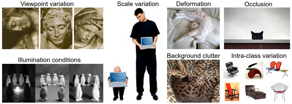
- Image classification problem has a lot of challenges like illumination and viewpoints.
- An image classification algorithm can be solved with K nearest neighborhood (KNN) but it can poorly solve the problem. The properties of KNN are:
- Hyperparameters can be optimized using Cross-validation as following (In our case we are trying tp predict K):
f folds.
2. Given predicted hyperparameters:
- Train your algorithm with f-1 folds and test it with the remain flood. and repeat this with every fold.
3. Choose the hyperparameters that gives the best training values (Average over all folds)
- Linear SVM classifier is an option for solving the image classification problem, but the curse of dimensions makes it stop improving at some point.
- Logistic regression is a also a solution for image classification problem, but image classification problem is non linear!
- Linear classifiers has to run the following equation:
Y = wX + b
w is the same as x and shape of b is 1.
- We can add 1 to X vector and remove the bias so that:
Y = wX
x is oldX+1 and w is the same as x
- We need to know how can we get
w's andb's that makes the classifier runs at best.
03. Loss function and optimization
- In the last section we talked about linear classifier but we didn't discussed how we could train the parameters of that model to get best
w's andb's.
- We need a loss function to measure how good or bad our current parameters.
Loss = L[i] =(f(X[i],W),Y[i])
Lossforall = 1/N * Sum(Li(f(X[i],W),Y[i])) # Indicates the average- Then we find a way to minimize the loss function given some parameters. This is called optimization.
- Loss function for a linear SVM classifier:
L[i] = Sum where all classes except the predicted class (max(0, s[j] - s[y[i]] + 1))
- We call this the hinge loss.
- Loss function means we are happy if the best prediction are the same as the true value other wise we give an error with 1 margin.
- Example:
- 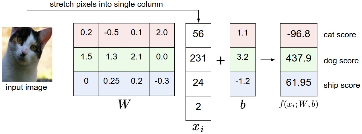 - Given this example we want to compute the loss of this image.
-
- Given this example we want to compute the loss of this image.
- L = max (0, 437.9 - (-96.8) + 1) + max(0, 61.95 - (-96.8) + 1) = max(0, 535.7) + max(0, 159.75) = 695.45
- Final loss is 695.45 which is big and reflects that the cat score needs to be the best over all classes as its the lowest value now. We need to minimize that loss.
- Its OK for the margin to be 1. But its a hyperparameter too.
- If your loss function gives you zero, are this value is the same value for your parameter? No there are a lot of parameters that can give you best score.
- You’ll sometimes hear about people instead using the squared hinge loss SVM (or L2-SVM). that penalizes violated margins more strongly (quadratically instead of linearly). The unsquared version is more standard, but in some datasets the squared hinge loss can work better.
- We add regularization for the loss function so that the discovered model don't overfit the data.
Loss = L = 1/N Sum(Li(f(X[i],W),Y[i])) + lambda R(W)- Where R is the regularizer, and lambda is the regularization term.
- There are different regularizations techniques:
R(W) = Sum(W^2) | Sum all the W squared |
| L1 | R(W) = Sum(lWl) | Sum of all Ws with abs |
| Elastic net (L1 + L2) | R(W) = beta * Sum(W^2) + Sum(lWl) | |
| Dropout | | No Equation |
- Regularization prefers smaller
Ws over bigWs.
- Regularizations is called weight decay. biases should not included in regularization.
- Softmax loss (Like linear regression but works for more than 2 classes):
-
A[L] = e^(score[L]) / sum(e^(score[L]), NoOfClasses)- Sum of the vector should be 1.
- Softmax loss:
-
Loss = -logP(Y = y[i]|X = x[i])- Log of the probability of the good class. We want it to be near 1 thats why we added a minus.
- Softmax loss is called cross-entropy loss.
- Consider this numerical problem when you are computing Softmax:
-
f = np.array([123, 456, 789]) # example with 3 classes and each having large scores       p = np.exp(f) / np.sum(np.exp(f)) # Bad: Numeric problem, potential blowup
# instead: first shift the values of f so that the highest number is 0:       f -= np.max(f) # f becomes [-666, -333, 0]       p = np.exp(f) / np.sum(np.exp(f)) # safe to do, gives the correct answer
- Optimization:
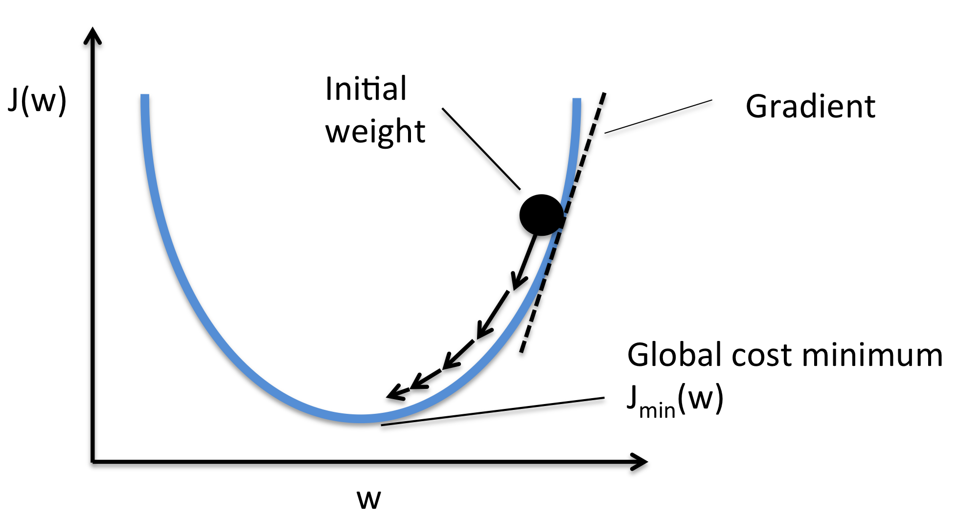 - Image source.
- Our goal is to compute the gradient of each parameter we have. - Numerical gradient: Approximate, slow, easy to write. (But its useful in debugging.) - Analytic gradient: Exact, Fast, Error-prone. (Always used in practice)
- After we compute the gradient of our parameters, we compute the gradient descent: -
W = W - learningrate * Wgrad- learning_rate is so important hyper parameter you should get the best value of it first of all the hyperparameters.
- stochastic gradient descent: - Instead of using all the date, use a mini batch of examples (32/64/128 are commonly used) for faster results.
04. Introduction to Neural network
- Computing the analytic gradient for arbitrary complex functions:
- Used to represent any function. with nodes. - Using Computational graphs can easy lead us to use a technique that called back-propagation. Even with complex models like CNN and RNN.
- Back-propagation simple example:
- Suppose we have f(x,y,z) = (x+y)z
- Then graph can be represented this way:
-
X \ (+)--> q ---(*)--> f / / Y / / / Z---------/- We made an intermediate variable q to hold the values of x+y
- Then we have:
-
q = (x+y) # dq/dx = 1 , dq/dy = 1 f = qz # df/dq = z , df/dz = q- Then:
-
df/dq = z df/dz = q df/dx = df/dq dq/dx = z 1 = z # Chain rule df/dy = df/dq dq/dy = z 1 = z # Chain rule- So in the Computational graphs, we call each operation f. For each f we calculate the local gradient before we go on back propagation and then we compute the gradients in respect of the loss function using the chain rule.
- In the Computational graphs you can split each operation to as simple as you want but the nodes will be a lot. if you want the nodes to be smaller be sure that you can compute the gradient of this node.
- A bigger example:
- 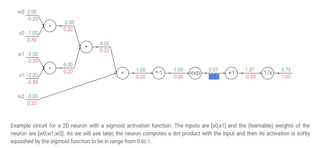 - Hint: the back propagation of two nodes going to one node from the back is by adding the two derivatives.
- Modularized implementation: forward/ backward API (example multiply code):
-
class MultuplyGate(object): """ x,y are scalars """ def forward(x,y): z = x*y self.x = x # Cache self.y = y # Cache # We cache x and y because we know that the derivatives contains them. return z def backward(dz): dx = self.y * dz #self.y is dx dy = self.x * dz return [dx, dy]- If you look at a deep learning framework you will find it follow the Modularized implementation where each class has a definition for forward and backward. For example:
- Multiplication - Max - Plus - Minus - Sigmoid - Convolution
- So to define neural network as a function:
f = Wx
- (Now) 2-layer neural network: f = W2max(0,W1x)
- Where max is the RELU non linear function
- (Now) 3-layer neural network: f = W3max(0,W2max(0,W1*x)
- And so on..
- Neural networks is a stack of some simple operation that forms complex operations.
05. Convolutional neural networks (CNNs)
- Neural networks history:
- Convolutional neural networks history:
- ConvNet architectures make the explicit assumption that the inputs are images, which allows us to encode certain properties into the architecture.
- There are a few distinct types of Layers in ConvNet (e.g. CONV/FC/RELU/POOL are by far the most popular)
- Each Layer may or may not have parameters (e.g. CONV/FC do, RELU/POOL don’t)
- Each Layer may or may not have additional hyperparameters (e.g. CONV/FC/POOL do, RELU doesn’t)
- How Convolutional neural networks works?
(X, M) the weighs shape for this will be (NoOfHiddenNeurons, X)
- Convolution layer is a layer in which we will keep the structure of the input by a filter that goes through all the image.
- We do this with dot product: W.T*X + b. This equation uses the broadcasting technique.
- So we need to get the values of W and b
- We usually deal with the filter (W) as a vector not a matrix.
- We call output of the convolution activation map. We need to have multiple activation map.
- Example if we have 6 filters, here are the shapes:
- Input image (32,32,3)
- filter size (5,5,3)
- We apply 6 filters. The depth must be three because the input map has depth of three.
- Output of Conv. (28,28,6)
- if one filter it will be (28,28,1)
- After RELU (28,28,6)
- Another filter (5,5,6)
- Output of Conv. (24,24,10)
- It turns out that convNets learns in the first layers the low features and then the mid-level features and then the high level features.
- After the Convnets we can have a linear classifier for a classification task.
- In Convolutional neural networks usually we have some (Conv ==> Relu)s and then we apply a pool operation to downsample the size of the activation.
- What is stride when we are doing convolution:
(7,7) and a filter with shape (3,3):
- If stride is 1 then the output shape will be (5,5) # 2 are dropped
- If stride is 2 then the output shape will be (3,3) # 4 are dropped
- If stride is 3 it doesn't work.
- A general formula would be ((N-F)/stride +1)
- If stride is 1 then O = ((7-3)/1)+1 = 4 + 1 = 5
- If stride is 2 then O = ((7-3)/2)+1 = 2 + 1 = 3
- If stride is 3 then O = ((7-3)/3)+1 = 1.33 + 1 = 2.33 # doesn't work
- In practice its common to zero pad the border.
# Padding from both sides.
1 its common to pad to this equation: (F-1)/2 where F is the filter size
- Example F = 3 ==> Zero pad with 1
- Example F = 5 ==> Zero pad with 2
- If we pad this way we call this same convolution.
- Adding zeros gives another features to the edges thats why there are different padding techniques like padding the corners not zeros but in practice zeros works!
- We do this to maintain our full size of the input. If we didn't do that the input will be shrinking too fast and we will lose a lot of data.
- Example:
(32,32,3) and ten filters with shape is (5,5) with stride 1 and pad 2
- Output size will be (32,32,10) # We maintain the size.
- Size of parameters per filter = 553 + 1 = 76
- All parameters = 76 * 10 = 76
- Number of filters is usually common to be to the power of 2.
# To vectorize well. - So here are the parameters for the Conv layer:
- Pooling makes the representation smaller and more manageable.
- Pooling Operates over each activation map independently.
- Example of pooling is the maxpooling.
2x2 with stride 2 # Usually the two parameters are the same 2 , 2
- Also example of pooling is average pooling.
06. Training neural networks I
- As a revision here are the Mini batch stochastic gradient descent algorithm steps:
- Activation functions:
- 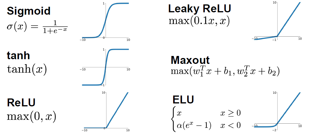
- Sigmoid:
- Squashes the numbers between [0,1] - Used as a firing rate like human brains. - Sigmoid(x) = 1 / (1 + e^-x) - Problems with sigmoid: - big values neurons kill the gradients. - Gradients are in most cases near 0 (Big values/small values), that kills the updates if the graph/network are large. - Not Zero-centered. - Didn't produce zero-mean data. - exp() is a bit compute expensive. - just to mention. We have a more complex operations in deep learning like convolution.
- Tanh:
- Squashes the numbers between [-1,1] - Zero centered. - Still big values neurons "kill" the gradients. - Tanh(x) is the equation. - Proposed by Yann Lecun in 1991.
- RELU (Rectified linear unit):
- RELU(x) = max(0,x) - Doesn't kill the gradients. - Only small values that are killed. Killed the gradient in the half - Computationally efficient. - Converges much faster than Sigmoid and Tanh (6x) - More biologically plausible than sigmoid. - Proposed by Alex Krizhevsky in 2012 Toronto university. (AlexNet) - Problems: - Not zero centered. - If weights aren't initialized good, maybe 75% of the neurons will be dead and thats a waste computation. But its still works. This is an active area of research to optimize this. - To solve the issue mentioned above, people might initialize all the biases by 0.01
- Leaky RELU:
- leaky_RELU(x) = max(0.01x,x) - Doesn't kill the gradients from both sides. - Computationally efficient. - Converges much faster than Sigmoid and Tanh (6x) - Will not die. - PRELU is placing the 0.01 by a variable alpha which is learned as a parameter.
- Exponential linear units (ELU):
-
ELU(x) = { x if x > 0 alpah *(exp(x) -1) if x <= 0 # alpah are a learning parameter }- It has all the benefits of RELU
- Closer to zero mean outputs and adds some robustness to noise.
- problems
- exp() is a bit compute expensive.
- Maxout activations:
- maxout(x) = max(w1.Tx + b1, w2.Tx + b2) - Generalizes RELU and Leaky RELU - Doesn't die! - Problems: - oubles the number of parameters per neuron
- In practice:
- Use RELU. Be careful for your learning rates. - Try out Leaky RELU/Maxout/ELU - Try out tanh but don't expect much. - Don't use sigmoid!
- Data preprocessing:
-
# Zero centered data. (Calculate the mean for every input).     # On of the reasons we do this is because we need data to be between positive and negative and not all the be negative or positive.      X -= np.mean(X, axis = 1)
# Then apply the standard deviation. Hint: in images we don't do this.     X /= np.std(X, axis = 1)
- To normalize images:
- Subtract the mean image (E.g. Alexnet) - Mean image shape is the same as the input images. - Or Subtract per-channel mean - Means calculate the mean for each channel of all images. Shape is 3 (3 channels)
- Weight initialization:
- All the neurons will do exactly the same thing. They will have the same gradient and they will have the same update. - So if W's of a specific layer is equal the thing described happened
- First idea is to initialize the w's with small random numbers:
-
W = 0.01 * np.random.rand(D, H) # Works OK for small networks but it makes problems with deeper networks!- The standard deviations is going to zero in deeper networks. and the gradient will vanish sooner in deep networks.
-
W = 1 * np.random.rand(D, H) # Works OK for small networks but it makes problems with deeper networks!- The network will explode with big numbers!
- Xavier initialization:
-
W = np.random.rand(in, out) / np.sqrt(in)- It works because we want the variance of the input to be as the variance of the output.
- But it has an issue, It breaks when you are using RELU.
- He initialization (Solution for the RELU issue):
-
W = np.random.rand(in, out) / np.sqrt(in/2)- Solves the issue with RELU. Its recommended when you are using RELU
- Proper initialization is an active area of research.
- Batch normalization:
Result = gamma * normalizedX + beta
- gamma and beta are learnable parameters.
- it basically possible to say “Hey!! I don’t want zero mean/unit variance input, give me back the raw input - it’s better for me.”
- Hey shift and scale by what you want not just the mean and variance!
- The algorithm makes each layer flexible (It chooses which distribution it wants)
- We initialize the BatchNorm Parameters to transform the input to zero mean/unit variance distributions but during training they can learn that any other distribution might be better.
- During the running of the training we need to calculate the globalMean and globalVariance for each layer by using weighted average.
- Benefits of Batch Normalization:
- Networks train faster.
- Allows higher learning rates.
- helps reduce the sensitivity to the initial starting weights.
- Makes more activation functions viable.
- Provides some regularization.
- Because we are calculating mean and variance for each batch that gives a slight regularization effect.
- In conv layers, we will have one variance and one mean per activation map.
- Batch normalization have worked best for CONV and regular deep NN, But for recurrent NN and reinforcement learning its still an active research area.
- Its challengey in reinforcement learning because the batch is small.
- Baby sitting the learning process
NAN then your NN exploded and your learning rate is high.
- Get your learning rate range by trying the min value (That can change) and the max value that doesn't explode the network.
7. Do Hyperparameters optimization to get the best hyperparameters values.
- Hyperparameter Optimization
07. Training neural networks II
- Optimization algorithms:
- if loss quickly in one direction and slowly in another (For only two variables), you will get very slow progress along shallow dimension, jitter along steep direction. Our NN will have a lot of parameters then the problem will be more. - Local minimum or saddle points - If SGD went into local minimum we will stuck at this point because the gradient is zero. - Also in saddle points the gradient will be zero so we will stuck. - Saddle points says that at some point: - Some gradients will get the loss up. - Some gradients will get the loss down. - And that happens more in high dimensional (100 million dimension for example) - The problem of deep NN is more about saddle points than about local minimum because deep NN has high dimensions (Parameters) - Mini batches are noisy because the gradient is not taken for the whole batch.
- SGD + momentum:
- Build up velocity as a running mean of gradients:
-
# Computing weighted average. rho best is in range [0.9 - 0.99] V[t+1] = rho * v[t] + dx x[t+1] = x[t] - learningRate * V[t+1]- V[0] is zero.
- Solves the saddle point and local minimum problems.
- It overshoots the problem and returns to it back.
- Nestrov momentum:
-
dx = compute_gradient(x) old_v = v v = rho v - learning_rate dx x+= -rho old_v + (1+rho) v- Doesn't overshoot the problem but slower than SGD + momentum
- AdaGrad
-
grad_squared = 0 while(True): dx = compute_gradient(x) # here is a problem, the grad_squared isn't decayed (gets so large) grad_squared += dx * dx x -= (learningrate*dx) / (np.sqrt(gradsquared) + 1e-7)- RMSProp
-
grad_squared = 0 while(True): dx = compute_gradient(x) #Solved ADAgra gradsquared = decayrate gradsquared + (1-gradsquared) dx * dx x -= (learningrate*dx) / (np.sqrt(gradsquared) + 1e-7)- People uses this instead of AdaGrad
- Adam
- Calculates the momentum and RMSProp as the gradients. - It need a Fixing bias to fix starts of gradients. - Is the best technique so far runs best on a lot of problems. - With beta1 = 0.9 and beta2 = 0.999 and learning_rate = 1e-3 or 5e-4 is a great starting point for many models!
- Learning decay
- Ex. decay learning rate by half every few epochs. - To help the learning rate not to bounce out. - Learning decay is common with SGD+momentum but not common with Adam. - Dont use learning decay from the start at choosing your hyperparameters. Try first and check if you need decay or not.
- All the above algorithms we have discussed is a first order optimization.
- Second order optimization
- Use gradient and Hessian to from quadratic approximation. - Step to the minima of the approximation. - What is nice about this update? - It doesn't has a learning rate in some of the versions. - But its unpractical for deep learning - Has O(N^2) elements. - Inverting takes O(N^3). - L-BFGS is a version of second order optimization - Works with batch optimization but not with mini-batches.
- In practice first use ADAM and if it didn't work try L-BFGS.
- Some says all the famous deep architectures uses SGS + Nestrov momentum
- Regularization
- Transfer learning:
- You need a lot of data if you want to train/use CNNs.
- Steps of transfer learning
1. Train on a big dataset that has common features with your dataset. Called pretraining. 2. Freeze the layers except the last layer and feed your small dataset to learn only the last layer. 3. Not only the last layer maybe trained again, you can fine tune any number of layers you want based on the number of data you have
- Guide to use transfer learning:
- | | Very Similar dataset | very different dataset | | ----------------------- | ---------------------------------- | ---------------------------------------- | | very little dataset | Use Linear classifier on top layer | You're in trouble.. Try linear classifier from different stages | | quite a lot of data | Finetune a few layers | Finetune a large layers |
- Transfer learning is the normal not an exception.
08. Deep learning software
- This section changes a lot every year in CS231n due to rabid changes in the deep learning softwares.
- CPU vs GPU
- Deep learning Frameworks
- Tensorflow (Google)
#Ships with tensorflow
- tf-Slim #Ships with tensorflow
- tf.contrib.learn #Ships with tensorflow
- Sonnet # New from deep mind
- Tensorflow has pretrained models that you can use while you are using transfer learning.
- Tensorboard adds logging to record loss, stats. Run server and get pretty graphs!
- It has distributed code if you want to split your graph on some nodes.
- Tensorflow is actually inspired from Theano. It has the same inspirations and structure.
- PyTorch (Facebook)
ndarray but runs on GPU #Like numpy arrays in tensorflow
- Variable: Node in a computational graphs; stores data and gradient #Like Tensor, Variable, Placeholders
- Module: A NN layer; may store state or learnable weights#Like tf.layers in tensorflow
- In PyTorch the graphs runs in the same loop you are executing which makes it easier for debugging. This is called a dynamic graph.
- In PyTorch you can define your own autograd functions by writing forward and backward for tensors. Most of the times it will implemented for you.
- Torch.nn is a high level api like keras in tensorflow. You can create the models and go on and on.
- You can define your own nn module!
- Also Pytorch contains optimizers like tensorflow.
- It contains a data loader that wraps a Dataset and provides minbatches, shuffling and multithreading.
- PyTorch contains the best and super easy to use pretrained models
- PyTorch contains Visdom that are like tensorboard. but Tensorboard seems to be more powerful.
- PyTorch is new and still evolving compared to Torch. Its still in beta state.
- PyTorch is best for research.
- Tensorflow builds the graph once, then run them many times (Called static graph)
- In each PyTorch iteration we build a new graph (Called dynamic graph)
- Static vs dynamic graphs:
- With static graphs, framework can optimize the graph for you before it runs.
- Serialization
- Static: Once graph is built, can serialize it and run it without the code that built the graph. Ex use the graph in c++
- Dynamic: Always need to keep the code around.
- Conditional
- Is easier in dynamic graphs. And more complicated in static graphs.
- Loops:
- Is easier in dynamic graphs. And more complicated in static graphs.
- Tensorflow fold make dynamic graphs easier in Tensorflow through dynamic batching.
- Dynamic graph applications include: recurrent networks and recursive networks.
- Caffe2 uses static graphs and can train model in python also works on IOS and Android
- Tensorflow/Caffe2 are used a lot in production especially on mobile.
09. CNN architectures
- This section talks about the famous CNN architectures. Focuses on CNN architectures that won ImageNet competition since 2012.
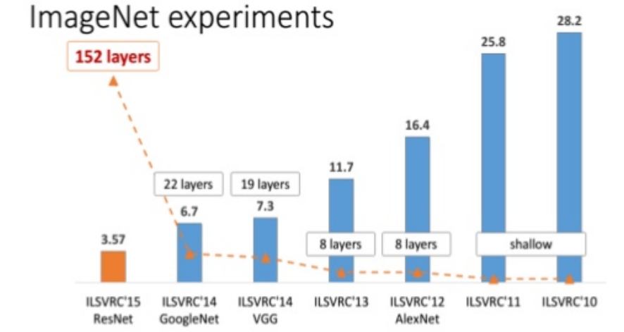
- Also we will discuss some interesting architectures as we go.
- The first ConvNet that was made was LeNet-5 architectures are:by Yann Lecun at 1998.
CONV-POOL-CONV-POOL-FC-FC-FC
- 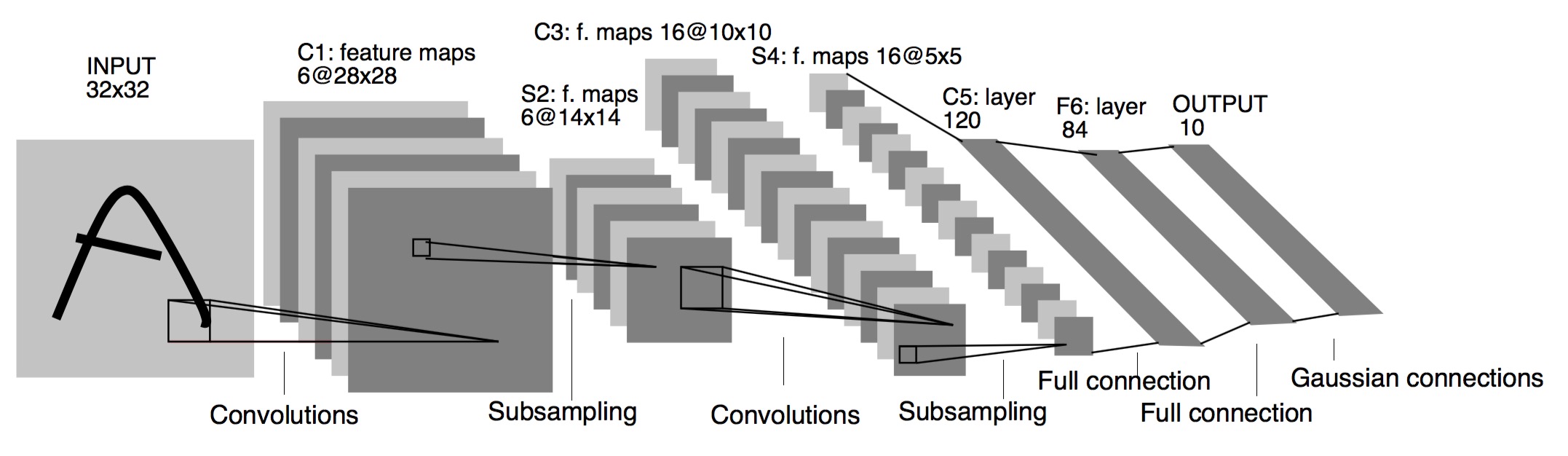 - Each conv filters was
 5x5 applied at stride 1
- Each pool was 2x2 applied at stride 2
- It was useful in Digit recognition.
- In particular the insight that image features are distributed across the entire image, and convolutions with learnable parameters are an effective way to extract similar features at multiple location with few parameters.
- It contains exactly 5 layers
- In 2010 Dan Claudiu Ciresan and Jurgen Schmidhuber published one of the very fist implementations of GPU Neural nets. This implementation had both forward and backward implemented on a a NVIDIA GTX 280 graphic processor of an up to 9 layers neural network.
- AlexNet (2012):
CONV1-MAXPOOL1-NORM1-CONV2-MAXPOOL2-NORM2-CONV3-CONV4-CONV5-MAXPOOL3-FC6-FC7-FC8
- Contains exactly 8 layers the first 5 are Convolutional and the last 3 are fully connected layers.
- AlexNet accuracy error was 16.4%
- For example if the input is 227 x 227 x3 then these are the shapes of the of the outputs at each layer:
- CONV1 (96 11 x 11 filters at stride 4, pad 0)
- Output shape (55,55,96), Number of weights are (11113*96)+96 = 34944
- MAXPOOL1 (3 x 3 filters applied at stride 2)
- Output shape (27,27,96), No Weights
- NORM1
- Output shape (27,27,96), We don't do this any more
- CONV2 (256 5 x 5 filters at stride 1, pad 2)
- MAXPOOL2 (3 x 3 filters at stride 2)
- NORM2
- CONV3 (384 3 x 3 filters ar stride 1, pad 1)
- CONV4 (384 3 x 3 filters ar stride 1, pad 1)
- CONV5 (256 3 x 3 filters ar stride 1, pad 1)
- MAXPOOL3 (3 x 3 filters at stride 2)
- Output shape (6,6,256)
- FC6 (4096)
- FC7 (4096)
- FC8 (1000 neurons for class score)
- Some other details:
- First use of RELU.
- Norm layers but not used any more.
- heavy data augmentation
- Dropout 0.5
- batch size 128
- SGD momentum 0.9
- Learning rate 1e-2 reduce by 10 at some iterations
- 7 CNN ensembles!
- AlexNet was trained on GTX 580 GPU with only 3 GB which wasn't enough to train in one machine so they have spread the feature maps in half. The first AlexNet was distributed!
- Its still used in transfer learning in a lot of tasks.
- Total number of parameters are 60 million
- ZFNet (2013)
CONV1: change from (11 x 11 stride 4) to (7 x 7 stride 2)
- CONV3,4,5: instead of 384, 384, 256 filters use 512, 1024, 512
- OverFeat (2013)
- VGGNet (2014) (Oxford)
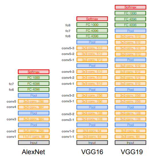
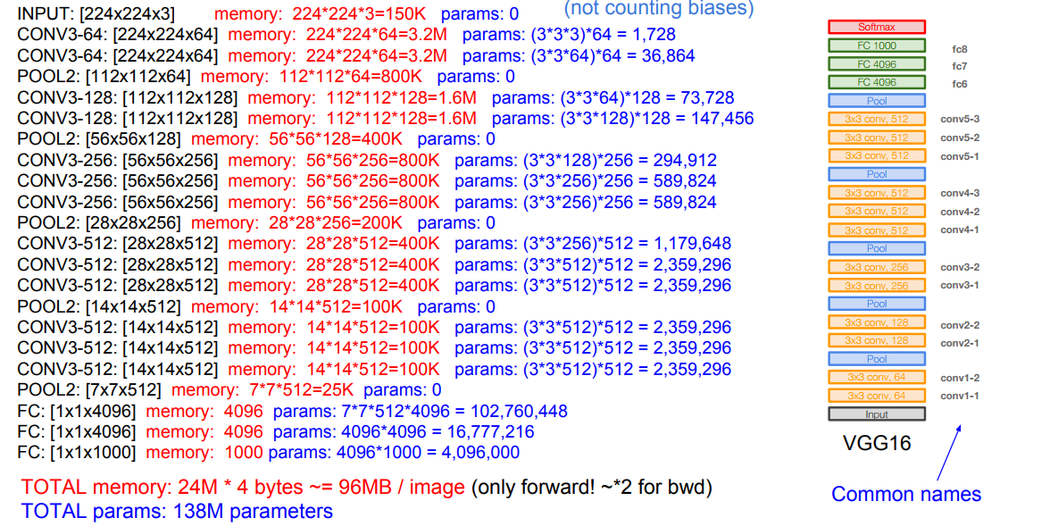 - The Architecture contains several CONV layers then POOL layer over 5 times and then the full connected layers.
- It has a total memory of 96MB per image for only forward propagation!
- Most memory are in the earlier layers
- Total number of parameters are 138 million
- Most of the parameters are in the fully connected layers
- Has a similar details in training like AlexNet. Like using momentum and dropout.
- VGG19 are an upgrade for VGG16 that are slightly better but with more memory
-
- The Architecture contains several CONV layers then POOL layer over 5 times and then the full connected layers.
- It has a total memory of 96MB per image for only forward propagation!
- Most memory are in the earlier layers
- Total number of parameters are 138 million
- Most of the parameters are in the fully connected layers
- Has a similar details in training like AlexNet. Like using momentum and dropout.
- VGG19 are an upgrade for VGG16 that are slightly better but with more memory
- 
- GoogleNet (2014)
# output shape (28,28,128)
- (3 x 3), 192 filter # output shape (28,28,192)
- (5 x 5), 96 filter # output shape (28,28,96)
- (3 x 3) Max pooling # output shape (28,28,256)
- After concatenation this will be (28,28,672)
- By this design -We call Naive- it has a big computation complexity.
- The last example will make:
- [1 x 1 conv, 128] ==> 28 28 128 1 1 * 256 = 25 Million approx
- [3 x 3 conv, 192] ==> 28 28 192 3 3 * 256 = 346 Million approx
- [5 x 5 conv, 96] ==> 28 28 96 5 5 * 256 = 482 Million approx
- In total around 854 Million operation!
- Solution: bottleneck layers that use 1x1 convolutions to reduce feature depth.
- Inspired from NiN (Network in network)
- 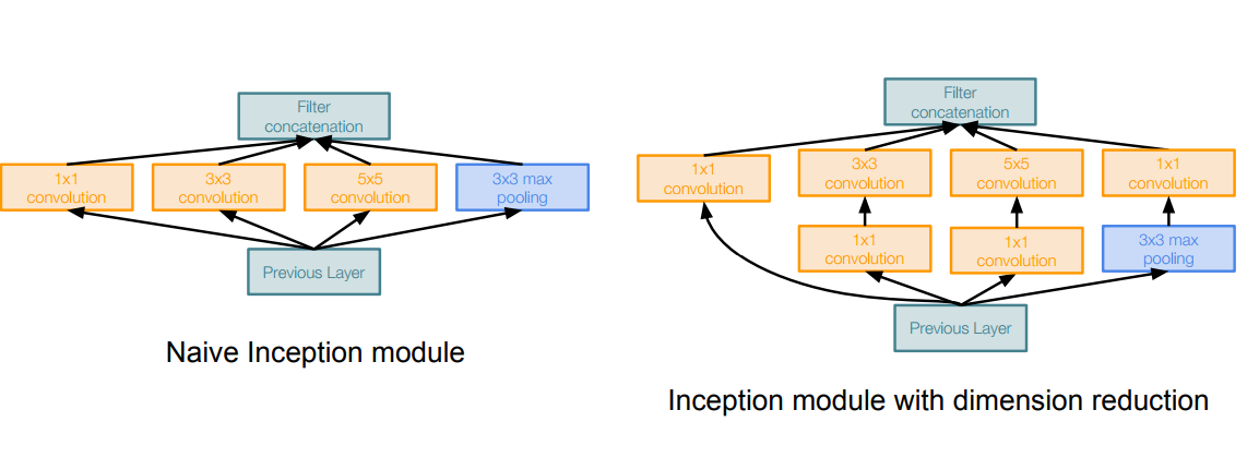 - The bottleneck solution will make a total operations of 358M on this example which is good compared with the naive implementation.
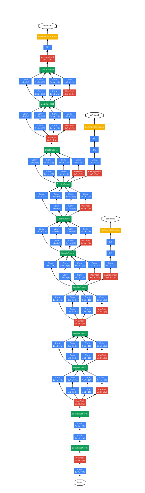
- So GoogleNet stacks this Inception module multiple times to get a full architecture of a network that can solve a problem without the Fully connected layers.
- Just to mention, it uses an average pooling layer at the end before the classification step.
- Full architecture:
-
- The bottleneck solution will make a total operations of 358M on this example which is good compared with the naive implementation.
- So GoogleNet stacks this Inception module multiple times to get a full architecture of a network that can solve a problem without the Fully connected layers.
- Just to mention, it uses an average pooling layer at the end before the classification step.
- Full architecture:
-  - In February 2015 Batch-normalized Inception was introduced as Inception V2. Batch-normalization computes the mean and standard-deviation of all feature maps at the output of a layer, and normalizes their responses with these values.
- In December 2015 they introduced a paper "Rethinking the Inception Architecture for Computer Vision" which explains the older inception models well also introducing a new version V3.
- In February 2015 Batch-normalized Inception was introduced as Inception V2. Batch-normalization computes the mean and standard-deviation of all feature maps at the output of a layer, and normalizes their responses with these values.
- In December 2015 they introduced a paper "Rethinking the Inception Architecture for Computer Vision" which explains the older inception models well also introducing a new version V3.
- The first GoogleNet and VGG was before batch normalization invented so they had some hacks to train the NN and converge well.
- ResNet (2015) (Microsoft Research)
- This is also the very first time that a network of > hundred, even 1000 layers was trained.
- Swept all classification and detection competitions in ILSVRC’15 and COCO’15!
- What happens when we continue stacking deeper layers on a “plain” Convolutional neural network?
- The deeper model performs worse, but it’s not caused by overfitting! - The learning stops performs well somehow because deeper NN are harder to optimize!
- The deeper model should be able to perform at least as well as the shallower model.
- A solution by construction is copying the learned layers from the shallower model and setting additional layers to identity mapping.
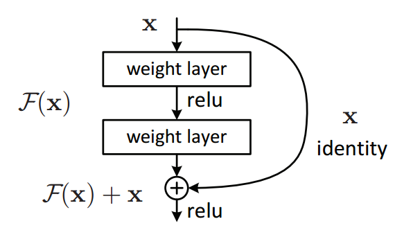
- Residual block:
- Microsoft came with the Residual block which has this architecture:
- 
-
# Instead of us trying To learn a new representation, We learn only Residual Y = (W2* RELU(W1x+b1) + b2) + X- Say you have a network till a depth of N layers. You only want to add a new layer if you get something extra out of adding that layer.
- One way to ensure this new (N+1)th layer learns something new about your network is to also provide the input(x) without any transformation to the output of the (N+1)th layer. This essentially drives the new layer to learn something different from what the input has already encoded.
- The other advantage is such connections help in handling the Vanishing gradient problem in very deep networks.
- With the Residual block we can now have a deep NN of any depth without the fearing that we can't optimize the network.
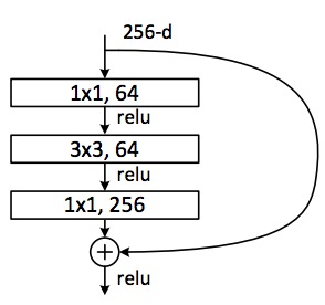
- ResNet with a large number of layers started to use a bottleneck layer similar to the Inception bottleneck to reduce the dimensions.
- 
- Full ResNet architecture:
- Stack residual blocks. - 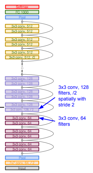 - Every residual block has two 3 x 3 conv layers. - Additional conv layer at the beginning. - No FC layers at the end (only FC 1000 to output classes) - Periodically, double number of filters and downsample spatially using stride 2 (/2 in each dimension) - Training ResNet in practice: - Batch Normalization after every CONV layer. - Xavier/2 initialization from He et al. - SGD + Momentum (
0.9) - Learning rate: 0.1, divided by 10 when validation error plateaus - Mini-batch size 256 - Weight decay of 1e-5 - No dropout used.
- Inception-v4: Resnet + Inception and was founded in 2016.
- The complexity comparing over all the architectures:
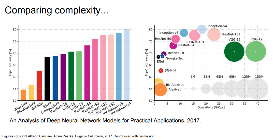 - VGG: Highest memory, most operations.
- GoogLeNet: most efficient.
- VGG: Highest memory, most operations.
- GoogLeNet: most efficient.
- ResNets Improvements:
- Beyond ResNets:
- Conclusion:
10. Recurrent Neural networks
- Vanilla Neural Networks "Feed neural networks", input of fixed size goes through some hidden units and then go to output. We call it a one to one network.
- Recurrent Neural Networks RNN Models:
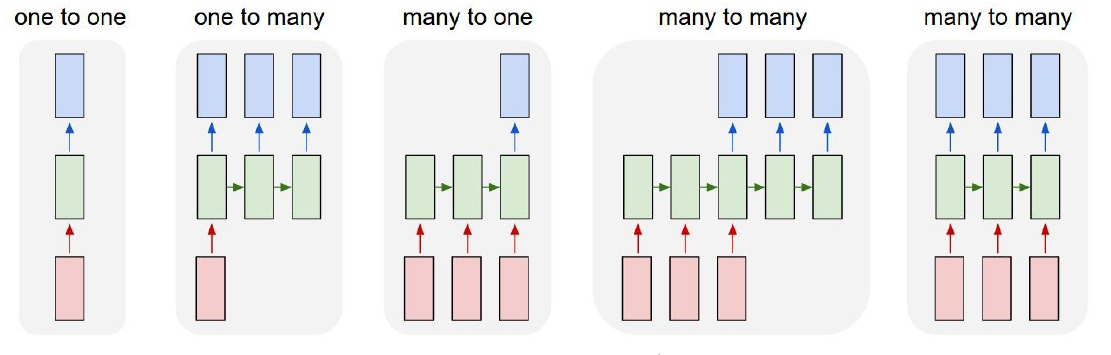 - One to many
- Example: Image Captioning
- image ==> sequence of words
- Many to One
- Example: Sentiment Classification
- sequence of words ==> sentiment
- Many to many
- Example: Machine Translation
- seq of words in one language ==> seq of words in another language
- Example: Video classification on frame level
- One to many
- Example: Image Captioning
- image ==> sequence of words
- Many to One
- Example: Sentiment Classification
- sequence of words ==> sentiment
- Many to many
- Example: Machine Translation
- seq of words in one language ==> seq of words in another language
- Example: Video classification on frame level
- RNNs can also work for Non-Sequence Data (One to One problems)
- So what is a recurrent neural network?
- 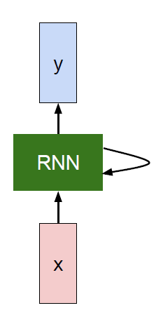
- The RNN block should return a vector.
- We can process a sequence of vectors x by applying a recurrence formula at every time step:
-
h[t] = fw (h[t-1], x[t]) # Where fw is some function with parameters W- The same function and the same set of parameters are used at every time step.
- (Vanilla) Recurrent Neural Network:
-
h[t] = tanh (W[h,h]h[t-1] + W[x,h]x[t]) # Then we save h[t] y[t] = W[h,y]*h[t]- This is the simplest example of a RNN.
- RNN works on a sequence of related data.
- Recurrent NN Computational graph:
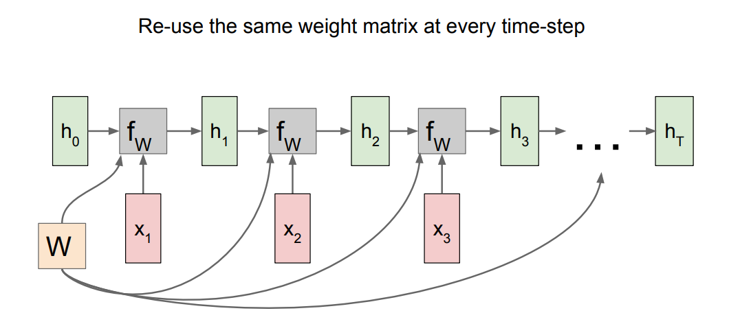 -
- h0 are initialized to zero.
- Gradient of W is the sum of all the W gradients that has been calculated!
- A many to many graph:
- 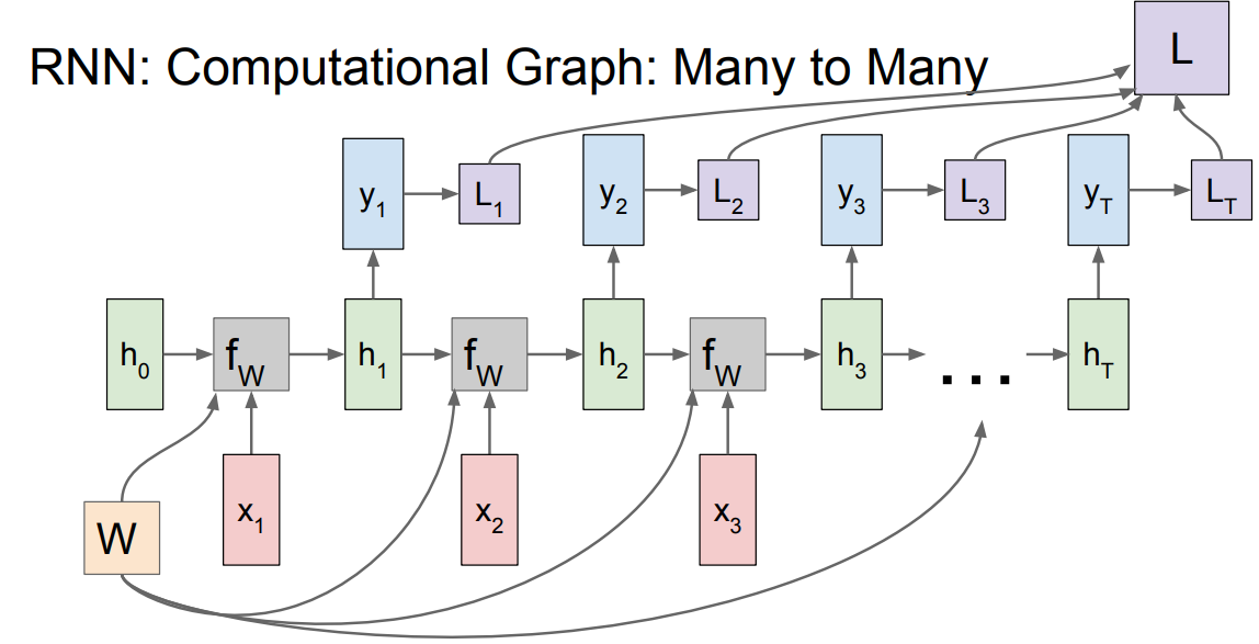 - Also the last is the sum of all losses and the weights of Y is one and is updated through summing all the gradients!
- A many to one graph:
-
- Also the last is the sum of all losses and the weights of Y is one and is updated through summing all the gradients!
- A many to one graph:
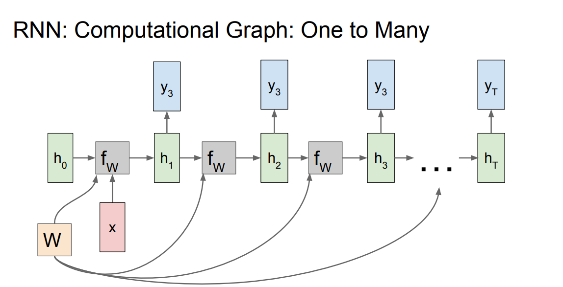
- 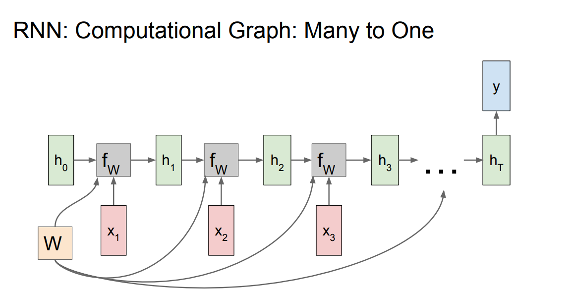 - A one to many graph:
-
- A one to many graph:
-  - sequence to sequence graph:
-
- sequence to sequence graph:
- 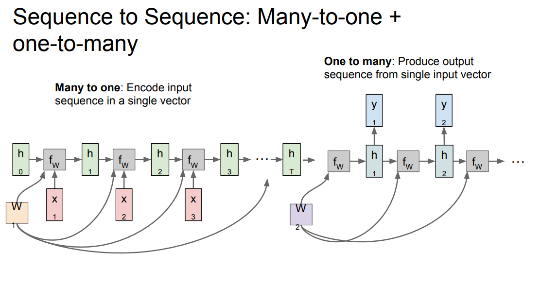 - Encoder and decoder philosophy.
- Examples:
[h, e, l, o] and the words are [hello]
- Training:
- 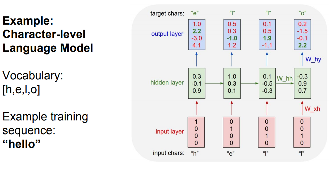 - Only the third prediction here is true. The loss needs to be optimized.
- We can train the network by feeding the whole word(s).
- Testing time:
-
- Only the third prediction here is true. The loss needs to be optimized.
- We can train the network by feeding the whole word(s).
- Testing time:
- 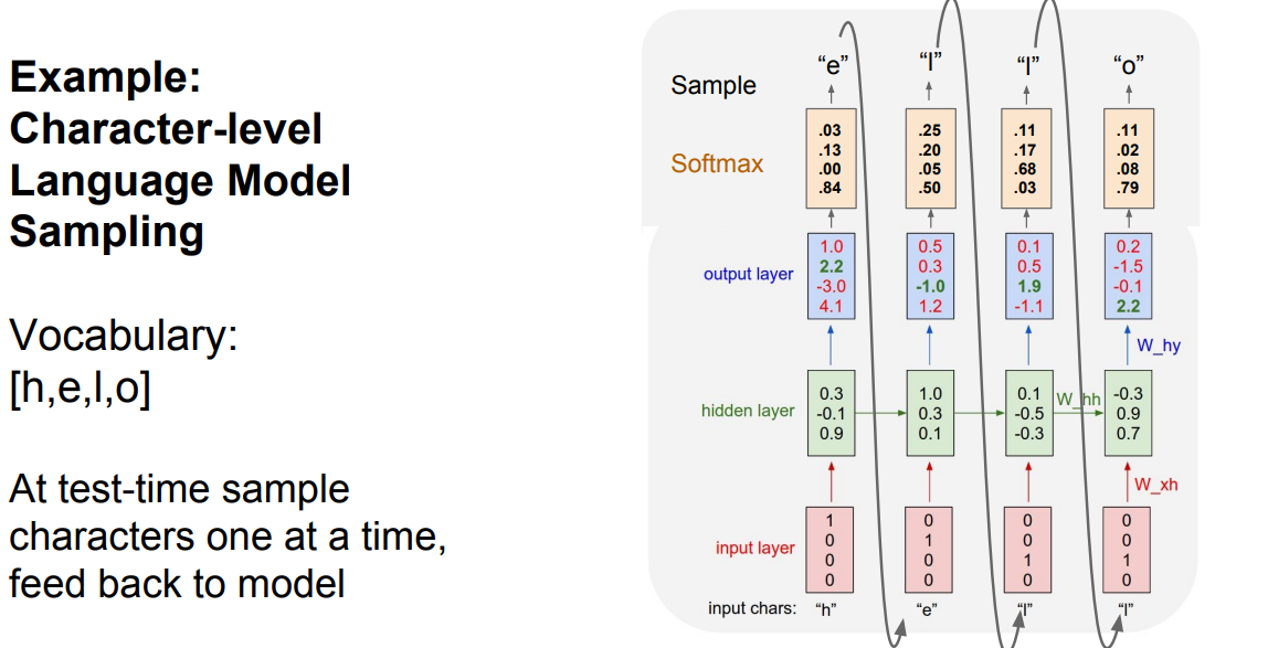 - At test time we work with a character by character. The output character will be the next input with the other saved hidden activations.
- This link contains all the code but uses Truncated Backpropagation through time as we will discuss.
- At test time we work with a character by character. The output character will be the next input with the other saved hidden activations.
- This link contains all the code but uses Truncated Backpropagation through time as we will discuss.
- Backpropagation through time Forward through entire sequence to compute loss, then backward through entire sequence to compute gradient.
- So in practice people are doing "Truncated Backpropagation through time" as we go on we Run forward and backward through chunks of the sequence instead of whole sequence
- Example on image captioning:
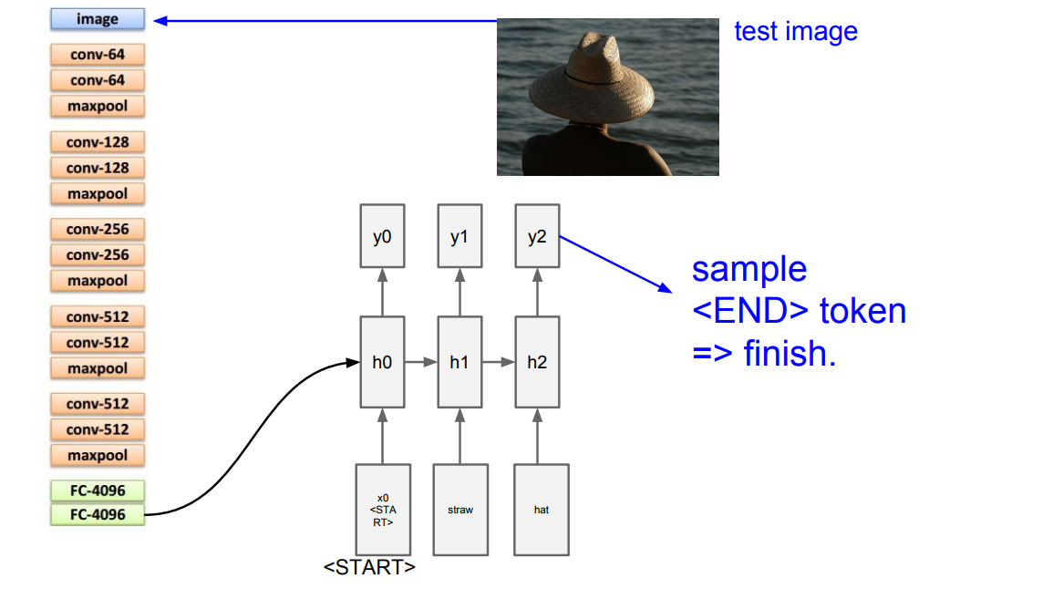 - They use
 - Image Captioning with Attention is a project in which when the RNN is generating captions, it looks at a specific part of the image not the whole image.
- Multilayer RNNs is generally using some layers as the hidden layer that are feed into again. LSTM is a multilayer RNNs.
- Backward flow of gradients in RNN can explode or vanish. Exploding is controlled with gradient clipping. Vanishing is controlled with additive interactions (LSTM)
- LSTM stands for Long Short Term Memory. It was designed to help the vanishing gradient problem on RNNs.
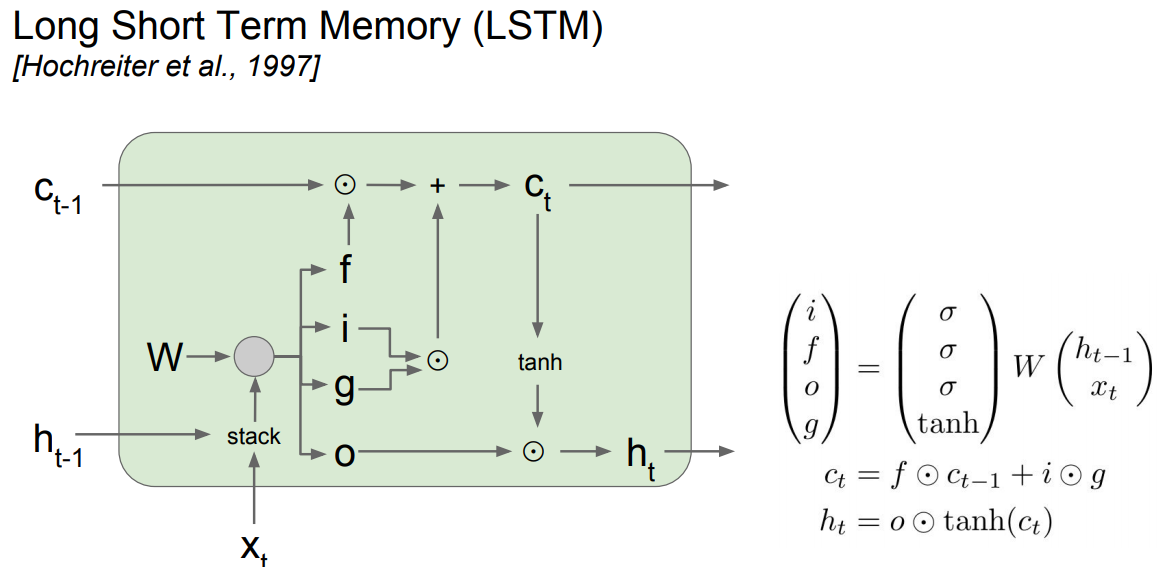 -
- 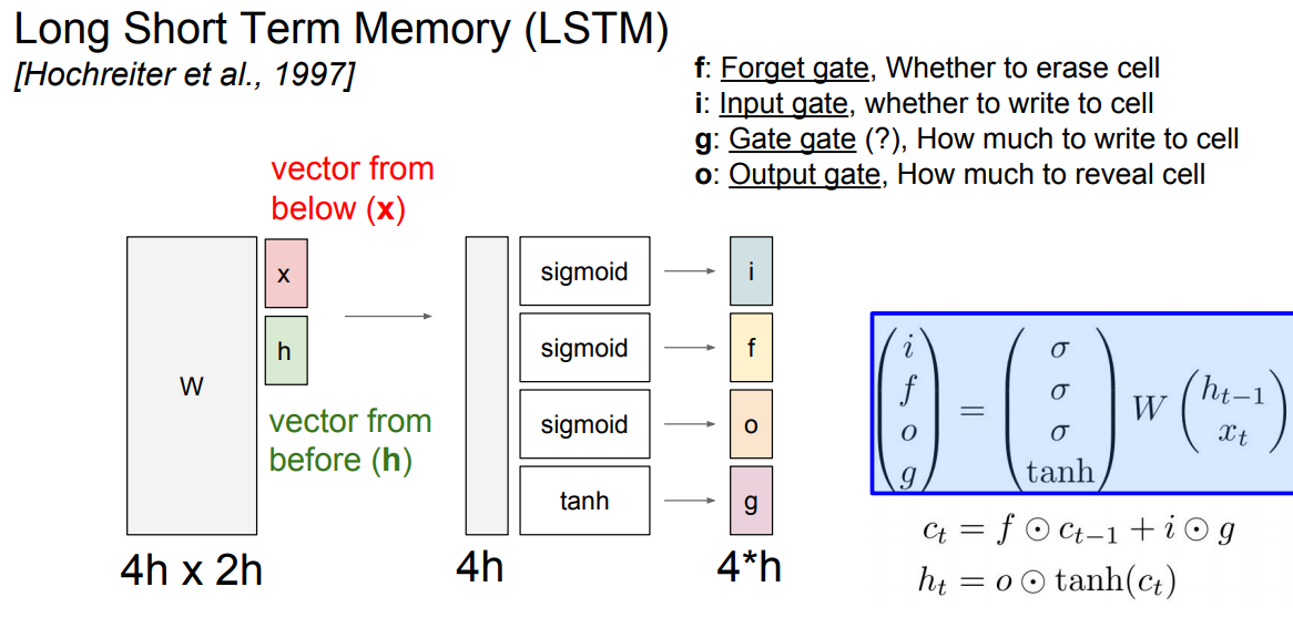 - The LSTM gradients are easily computed like ResNet
- The LSTM is keeping data on the long or short memory as it trains means it can remember not just the things from last layer but layers.
- The LSTM gradients are easily computed like ResNet
- The LSTM is keeping data on the long or short memory as it trains means it can remember not just the things from last layer but layers.
- Highway networks is something between ResNet and LSTM that is still in research.
- Better/simpler architectures are a hot topic of current research
- Better understanding (both theoretical and empirical) is needed.
- R
README truncated. View on GitHub


