Topics

#mode #mode-solver #photonic-mode-solver #photonics #python #python2 #python3 #waveguide

Language breakdown

Python 100.0%

▸ Files click to expand

README

modesolverpy

Photonic mode solver with a nice interface and output.

semi-vectorial and fully vectorial options,
simple structure drawing,
automated data saving and plotting via Gnuplot,
some limited (at this stage) data processing (finding MFD of fundamental mode), and
easily extensible library

The documentation for this project can be found here.

Examples

Ex1: Semi-vectorial mode solving of a ridge waveguide
Ex2: Fully vectorial mode solving of an anisotropic material waveguide
Ex3: Grating-coupler period
Ex4: Mode Hybridisation In SOI
Ex6: Directional Coupler 3dB Length In SOI

Example 1: Semi-vectorial mode solving of a ridge waveguide

The following example finds the first two modes of a waveguide with the following, arbitrary, parameters:

thin-film thickness: 500nm
waveguide height: 400nm,
waveguide width: 500nm,
refractive index of waveguide: 3,
refractive index of substrate: 1.4,
refractive index of cladding: 1, and
wavelength: 1550nm.

Python script

import modesolverpy.mode_solver as ms
import modesolverpy.structure as st
import numpy as np
All units are relative.  [um] were chosen in this case.
x_step = 0.02
y_step = 0.02
wg_height = 0.4
wg_width = 0.5
sub_height = 0.5
sub_width = 2.
clad_height = 0.5
n_sub = 1.4
n_wg = 3.
n_clad = 1.
film_thickness = 0.5
wavelength = 1.55
angle = 75.
structure = st.RidgeWaveguide(wavelength,                               x_step,                               y_step,                               wg_height,                               wg_width,                               sub_height,                               sub_width,                               clad_height,                               n_sub,                               n_wg,                               angle,                               n_clad,                               film_thickness)
structure.writetofile('examplestructure1.dat')
modesolver = ms.ModeSolverSemiVectorial(2, semivectorial_method='Ey') mode_solver.solve(structure) modesolver.writemodestofile('examplemodes1.dat')

Structure

Modes

Example 2: Fully vectorial mode solving of an anisotropic material waveguide

The following looks at a contrived ridge waveguide in Z-cut KTP.

The simulation outputs:

5 plots for each refractive index axis (nxx, nxy, nyx, nyy and n_zz),
48 plots for Ex, Ey, Ez, Hx, Hy and Hz,
8 effective index values, one for each mode,
a wavelength sweep of the waveguide (plotting n_eff vs wavelength for each mode),
whether a mode is qTE or qTM and the percentage overlap with TE and TM, and
the group velocity of the mode.

The waveguide parameters are:

thin-film thickness: 1.2um,
waveguide height: 800nm,
waveguide width: 1.2um,
refractive index of waveguide: used Sellmeier equations to get nxx, nyy, n_zz at 1550nm,
refractive index of substrate: used Sellmeier equation to get SiO2 at 1550nm,
refractive index of cladding: 1, and
wavelength: 1550nm.

Python script

import modesolverpy.mode_solver as ms import modesolverpy.structure as st import opticalmaterialspy as mat import numpy as np
wl = 1.55 x_step = 0.06 y_step = 0.06 wg_height = 0.8 wg_width = 1.8 sub_height = 1.0 sub_width = 4. clad_height = 1.0 film_thickness = 1.2 angle = 60.
def structfunc(nsub, nwg, nclad):     return st.RidgeWaveguide(wl, xstep, ystep, wgheight, wgwidth,                              subheight, subwidth, clad_height,                              nsub, nwg, angle, nclad, filmthickness)
n_sub = mat.SiO2().n(wl) nwgxx = mat.Ktp('x').n(wl) nwgyy = mat.Ktp('y').n(wl) nwgzz = mat.Ktp('z').n(wl) n_clad = mat.Air().n()
structxx = structfunc(nsub, nwgxx, nclad) structyy = structfunc(nsub, nwgyy, nclad) structzz = structfunc(nsub, nwgzz, nclad)
structani = st.StructureAni(structxx, structyy, structzz) structani.writeto_file()
solver = ms.ModeSolverFullyVectorial(8) solver.solve(struct_ani) solver.writemodesto_file()
solver.solveng(structani, 1.55, 0.01)
solver.solvesweepwavelength(struct_ani, np.linspace(1.501, 1.60, 21))

Group Velocity

The group velocity at 1550nm for each mode is:

# modesfullvec/ng.dat
Mode idx, Group index
0,1.776
1,1.799
2,1.826
3,1.847
4,1.841
5,1.882
6,1.872
7,1.871

Structure

Modes

Only the first 4 (out of 8) modes are shown, and only the E-fields are shown (not H-fields). For the rest of the images, look in the example folder or run the script.

A_{x,y,z} give the percentage power of that particular E-field component with respect to the total of all components.

Mode types:

# modesfullvec/mode_info Mode idx, Mode type, % in major direction, n_eff
 0,qTE,97.39,1.643 1,qTM,92.54,1.640 2,qTE,90.60,1.576 3,qTM,91.41,1.571 4,qTE,89.48,1.497 5,qTM,86.70,1.475 6,qTE,89.47,1.447 7,qTM,68.35,1.437

Wavelength Sweep

Example 3: Grating-coupler period

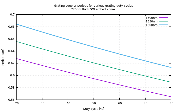
Analytic calculation of the grating coupler period for various duty-cycles in SOI.

Seems to match well with the periods in Taillaert et al., Grating Couplers for Coupling between Optical Fibers and Nanophotonic Waveguides_, IOP Science, 2006.

import modesolverpy.mode_solver as ms
import modesolverpy.structure as st
import modesolverpy.design as de
import opticalmaterialspy as mat
import numpy as np
wls = [1.5, 1.55, 1.6] x_step = 0.05 y_step = 0.05 etch_depth = 0.07 wg_width = 10 sub_height = 0.5 sub_width = 14. clad_height = 0.5 film_thickness = 0.22 polarisation = 'TE' dcs = np.linspace(20, 80, 61) / 100
ed1 = etch_depth ft1 = film_thickness ed2 = ft1 - ed1 ft2 = ed2
periods = [] periods.append(dcs)
for wl in wls:     ngc = []     for ed, ft in [(ed1, ft1), (ed2, ft2)]:         def structfunc(nsub, nwg, nclad):             return st.RidgeWaveguide(wl, xstep, ystep, ed, wg_width,                                      subheight, subwidth, clad_height,                                      nsub, nwg, None, n_clad, ft)
n_sub = mat.SiO2().n(wl)         nwgxx = 3.46         nwgyy = 3.46         nwgzz = 3.46         n_clad = mat.Air().n()
structxx = structfunc(nsub, nwgxx, nclad)         structyy = structfunc(nsub, nwgyy, nclad)         structzz = structfunc(nsub, nwgzz, nclad)
structani = st.StructureAni(structxx, structyy, structzz)         #structani.writeto_file()
solver = ms.ModeSolverFullyVectorial(4)         solver.solve(struct_ani)         #solver.writemodesto_file()
if polarisation == 'TE':             ngc.append(np.round(np.real(solver.neffste), 4)[0])         elif polarisation == 'TM':             ngc.append(np.round(np.real(solver.neffstm), 4)[0])
period = de.gratingcouplerperiod(wl, dcsngc[0]+(1-dcs)ngc[1], n_clad, 8, 1)     periods.append(period)
filename = 'dc-sweep-%s-%inm-etch-%i-film.dat' % (polarisation, etchdepth1000, filmthickness1000) np.savetxt(filename, np.array(periods).T, delimiter=',', header=','.join([str(val) for val in wls])) print(np.c_[periods])

Example 4: Mode Hybridisation In SOI

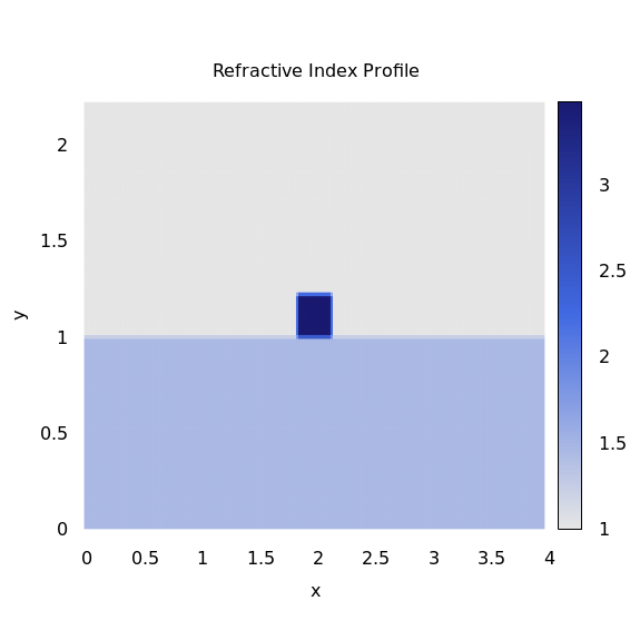
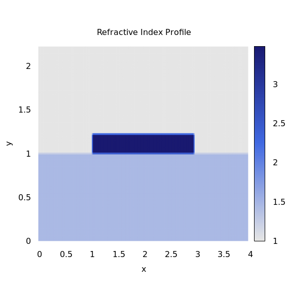
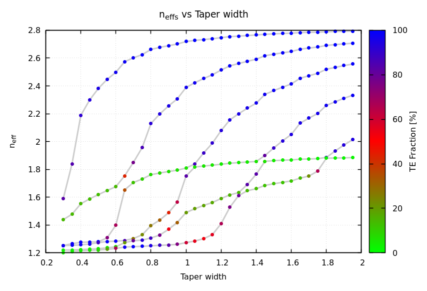
Simulation of mode hybridisation in 220nm thick fully-etched SOI ridge waveguides.

Results look the same as those found in Daoxin Dai and Ming Zhang, "Mode hybridization and conversion in silicon-on-insulator nanowires with angled sidewalls," Opt. Express 23, 32452-32464 (2015).

import modesolverpy.mode_solver as ms
import modesolverpy.structure as st
import opticalmaterialspy as mat
import numpy as np
wl = 1.55 x_step = 0.02 y_step = 0.02 etch_depth = 0.22 wg_widths = np.arange(0.3, 2., 0.05) sub_height = 1. sub_width = 4. clad_height = 1. film_thickness = 0.22
n_sub = mat.SiO2().n(wl) n_clad = mat.Air().n(wl) n_wg = mat.RefractiveIndexWeb(     'https://refractiveindex.info/?shelf=main&book=Si&page=Li-293K').n(wl)
r = [] for w in wg_widths:     r.append(         st.RidgeWaveguide(wl, xstep, ystep, etchdepth, w, subheight,                           subwidth, cladheight, nsub, nwg, None, n_clad,                           film_thickness))
r[0].writetofile('startnprofile.dat') r[-1].writetofile('endnprofile.dat')
solver = ms.ModeSolverFullyVectorial(6) solver.solvesweepstructure(r, wgwidths, xlabel='Taper width', fractionmodelist=[1,2]) solver.writemodesto_file()

Example 5: Directional Coupler 3dB Length In SOI

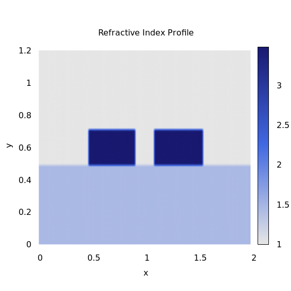
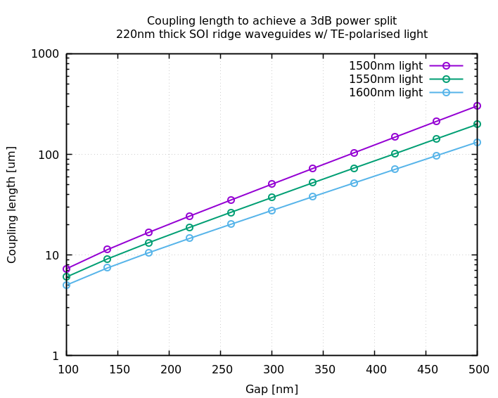
Analytic calculation of 3dB coupling length into two parallel SOI waveguides with a varying gap at 3 different TE wavelengths.

An example refractive index profile for the two waveguides spaced 200nm is shown.

import modesolverpy.mode_solver as ms
import modesolverpy.structure as st
import modesolverpy.design as de
import opticalmaterialspy as mat
import numpy as np
import tqdm
wls = [1.5, 1.55, 1.6] x_step = 0.02 y_step = 0.02 etch_depth = 0.22 wg_width = 0.44 sub_height = 0.5 sub_width = 2. clad_height = 0.5 film_thickness = 0.22 gaps = np.linspace(0.1, 0.5, 11)
for wl in wls:     lengths = []
n_sub = mat.SiO2().n(wl)     n_clad = mat.Air().n(wl)     n_wg = 3.476
for gap in tqdm.tqdm(gaps):         r = st.WgArray(wl, xstep, ystep, etchdepth, [wgwidth, wg_width], gap,                        subheight, subwidth, cladheight, nsub, n_wg, None)         #r.writetofile()
solver = ms.ModeSolverFullyVectorial(2)         solver.solve(r)         n1 = solver.neffste[0]         n2 = solver.neffste[1]         lengths.append(de.directionalcouplerlc(wl*1000, n1, n2)/2)
filename = 'dc-sweep-%inm-%s-%inm-etch-%i-film.dat' % (wl1000, 'TE', etchdepth1000, filmthickness*1000)     np.savetxt(filename, np.c_[gaps, lengths], delimiter=',', header='Coupling lengths (50\%)')

Installation

It is recommend to install modesolverpy either via:

Ubuntu/Mint/Debian:

pip3 install modesolverpy # or pip2 install modesolverpy
apt install gnuplot

Arch Linux:

yaourt -S python-modesolverpy

Dependencies

If installing using the Arch Linux AUR package or pip, dependencies will be automatically downloaded and installed, if not, one should ensure the following dependencies are installed:

Either Gnuplot or Matplotlib can be used for plotting; I am a Gnuplot user to the code was written with it in mind. If both Gnuplot and Matplotlib are installed, the code will default to Gnuplot.