Topics

#algorithmic-trading #backpropagation-through-time #cryptocurrency #deep-learning #differentiable-programming #itransformer #pytorch #quantitative-finance #reinforcement-learning #sharpe-ratio #time-series-forecasting

Language breakdown

No language data available.

▸ Files click to expand

README

DiffQuant

End-to-End Differentiable Trading Pipeline

How it works

The full pipeline is a single differentiable computation graph:

features[t−ctx:t] → PolicyNetwork → position_t → DiffSimulator → −Sharpe → ∂/∂θ

The simulator implements exact mark-to-market accounting as tensor operations — no surrogate losses, no reward shaping. The entire chain is differentiable:

rett      = (closet − close{t−1}) / close{t−1}
grosst    = position{t−1} × ret_t
costt     = smoothabs(Δpos_t) × (commission + slippage)
netpnlt  = grosst − costt

smooth_abs(x) = √(x² + ε) replaces |x| to preserve C∞ differentiability through transaction cost computation — critical when the model operates near flat.

Policy head: direction × gate

position = tanh(directionraw / τdir) × sigmoid(gateraw / τgate)

direction encodes the alpha signal; gate encodes whether to trade at all. When confidence is low, gate → 0 and position → 0 regardless of direction — the differentiable analogue of action masking. Gate bias is initialized to −1.0, so the model starts in a near-flat regime and opens positions only when accumulated gradient evidence justifies the exposure. This stabilizes early training when policy outputs are noisy.

Training objective

L = λ₁·(−Sharpe) + λ₂·turnover + λ₃·drawdown + λ₄·terminal + λ₅·(flatsoft − flattarget)² + λ₆·|mean(pos)|

Each term addresses a specific failure mode: turnover prevents commission drag; drawdown discourages extended underwater periods; terminal penalizes open risk at episode end; flat_target prevents permanent flat collapse; bias penalizes always-long or always-short behavior, which proved critical for symmetric long/short learning on trending BTC training data.

Validation protocol

Both training validation and backtest use continuous walk-forward evaluation, identical to live execution mechanics:

for t in range(ctx_len, N):
    window   = features[t − ctx : t]       # past ctx bars only
    position = model(normalize(window))     # single forward pass
    pnlt    = prevpos × ret_t − commission × |Δpos|
    # position carried to next bar — no resets

The same WalkForwardEvaluator runs during training (every val_freq epochs) and at final evaluation. There is no separate validation logic anywhere else in the codebase. This is intentional.

Quick start

git clone https://github.com/YuriyKolesnikov/diffquant
cd diffquant
pip install -r requirements.txt
Download 1-min BTCUSDT 2021–2025 from HuggingFace
huggingface-cli download ResearchRL/diffquant-data --local-dir data_source/ --repo-type dataset
Verify gradient flow and trend learning before training
python sanitycheck.py --config configs/experiments/itransformerhybrid.py
Expected output:
  PASS  gradient_flow    all params receive gradient
  PASS  longbias        meanposition=+0.19  expected_sign=+
  PASS  shortbias       meanposition=-0.16  expected_sign=-
  ALL PASSED
Train primary experiment
python train.py --config configs/experiments/itransformer_hybrid.py --device cuda
Optional: find optimal thresholds on the val set
python optimizethresholds.py --config configs/experiments/itransformerhybrid.py --trials 100 --objective sharpe
Evaluate on held-out test and backtest splits
python evaluate.py --config configs/experiments/itransformer_hybrid.py
Evaluate with final model checkpoint
python evaluate.py --config configs/experiments/itransformerhybrid.py --checkpoint output/itransformerhybrid/models/final.pth
Hyperparameter search
python optimize.py --config configs/experiments/itransformer_hybrid.py --trials 100
Compare all completed experiments
python compare.py

Structure

diffquant/
├── configs/
│   ├── base_config.py          # MasterConfig — single source of all hyperparameters
│   └── experiments/            # One file per experiment; overrides selectively
├── data/
│   ├── pipeline.py             # loadorbuild() — MD5-cached dataset construction
│   ├── aggregator.py           # 1-min → N-min, clock-aligned resampling
│   ├── features.py             # Log-returns, volume ratios, cyclic time encoding
│   ├── splitter.py             # Temporal split by datetime boundary
│   ├── dataset.py              # TradingDataset (full ctx+hor sequences)
│   └── normalization.py        # Per-sample z-score, no look-ahead
├── model/
│   ├── backbone/
│   │   ├── itransformer.py     # Channel-wise attention (Liu et al., ICLR 2024)
│   │   └── lstm_encoder.py     # Bidirectional LSTM encoder
│   ├── policy_head.py          # direction × gate two-headed output
│   └── policy_network.py       # Backbone + head → position ∈ (−1, +1)
├── simulator/
│   ├── diffsimulator.py       # Mark-to-market PnL, smoothabs, SimConfig
│   └── losses.py               # sharpe / sortino / hybrid
├── training/
│   └── trainer.py              # DiffTrainer — episode rollout + walk-forward val
├── evaluation/
│   ├── walk_forward.py         # Continuous evaluation engine (val + backtest)
│   └── backtest.py             # Full reporting wrapper
├── utils/
│   ├── metrics.py              # All financial metrics — one location
│   ├── logging_utils.py        # MetricsLogger — val JSONL + full reports
│   ├── utils.py                # Auxiliary functions
│   └── visualization.py        # Equity curves, position distribution
├── sanity/
│   └── checks.py               # Gradient flow + trend bias checks
├── train.py
├── evaluate.py
├── sanity_check.py
├── optimize.py                 # Optuna hyperparameter search
├── optimize_thresholds.py      # Optuna threshold selection on val
└── compare.py                  # Experiment comparison table

Experiments

| Config | Backbone | Loss | Purpose | |---|---|---|---| | itransformer_sharpe | iTransformer | −Sharpe only | Ablation: loss function contribution | | itransformer_hybrid | iTransformer | Hybrid | Primary experiment | | lstm_hybrid | LSTM (bidir.) | Hybrid | Backbone comparison |

The three configs share the same data, simulator, and evaluation protocol. Any performance difference is attributable to architecture or loss function alone.

Configuration

# Minimal override example
from configs.base_config import MasterConfig
cfg = MasterConfig(experimentname="itransformerhybrid") cfg.backbone.type           = "itransformer" cfg.loss.type               = "hybrid" cfg.loss.lambda_turnover    = 0.01 cfg.loss.lambda_bias        = 0.25          # penalises always-long / always-short cfg.loss.lambdaflattarget = 0.5           # prevents permanent flat collapse cfg.data.preset             = "ohlcv"       # open, high, low, close, volume cfg.data.addrollingvol    = True          # causal rolling volatility channel cfg.data.timeframe_min      = 30            # aggregate 1-min source to 30-min bars

Feature presets: "ohlc" | "ohlcv" (default) | "full" | "custom".

Dataset

| | | |---|---| | Asset | BTCUSDT Binance Futures (USDⓈ-M perpetual) | | Source resolution | 1-minute bars (close-time convention) | | HuggingFace | ResearchRL/diffquant-data | | Period | 2021-01-01 — 2025-12-31 |

Dataset: HuggingFace Hub

Temporal splits (all non-overlapping):

| Split | Period | Purpose | |---|---|---| | Train | 2024-01-01 → 2025-03-31 | Gradient updates | | Val | 2025-04-01 → 2025-06-30 | Model selection during training | | Test | 2025-07-01 → 2025-09-30 | Out-of-sample evaluation | | Backtest | 2025-10-01 → 2025-12-31 | Final held-out evaluation |

Aggregation from 1-min to any target timeframe uses origin="epoch" alignment, ensuring bars always land on clock boundaries (:00, :05, :10, … for 5-min). The primary experiment uses 30-min bars: context = 96 bars (48 hours), horizon = 24 bars (12 hours).

The training window is intentionally limited to 15 months (January 2024 – March 2025) rather than the full historical record. This keeps the training regime temporally close to the evaluation periods and minimises distribution shift. Extending to earlier data is straightforward via SplitConfig.train_start and is the recommended first ablation.

Experimental status

DiffQuant is an active research project. The results below represent the first promising configuration found during initial experimentation. The pipeline is hyperparameter-sensitive — loss weights, learning rate, training window, and feature composition interact non-trivially. Results vary across configurations and market regimes. The codebase is designed to support systematic reproduction and further experimentation.

This is research, not a production-ready system.

Results

Experiment: `itransformer_hybrid`

Configuration summary:

Backbone: iTransformer (dmodel=32, nlayers=4) — 52K parameters
Features: ohlcv + rolling_vol (6 channels), 30-min bars
Training data: Jan 2024 → Mar 2025 (15 months, 910 non-overlapping samples)
Loss: Hybrid (Sharpe + drawdown + flat_target + bias)
Training: 30 epochs, lr=1e-3, mirror_augmentation=True

Why a small model and non-overlapping samples: 910 training samples is intentionally small. With stride=horizon_len=24, each sample covers a distinct 12-hour market window with no overlap, preventing the model from memorizing sequential price paths. A 52K-parameter model on 910 independent episodes is deliberately capacity-constrained to resist microstructure noise.

Training dynamics

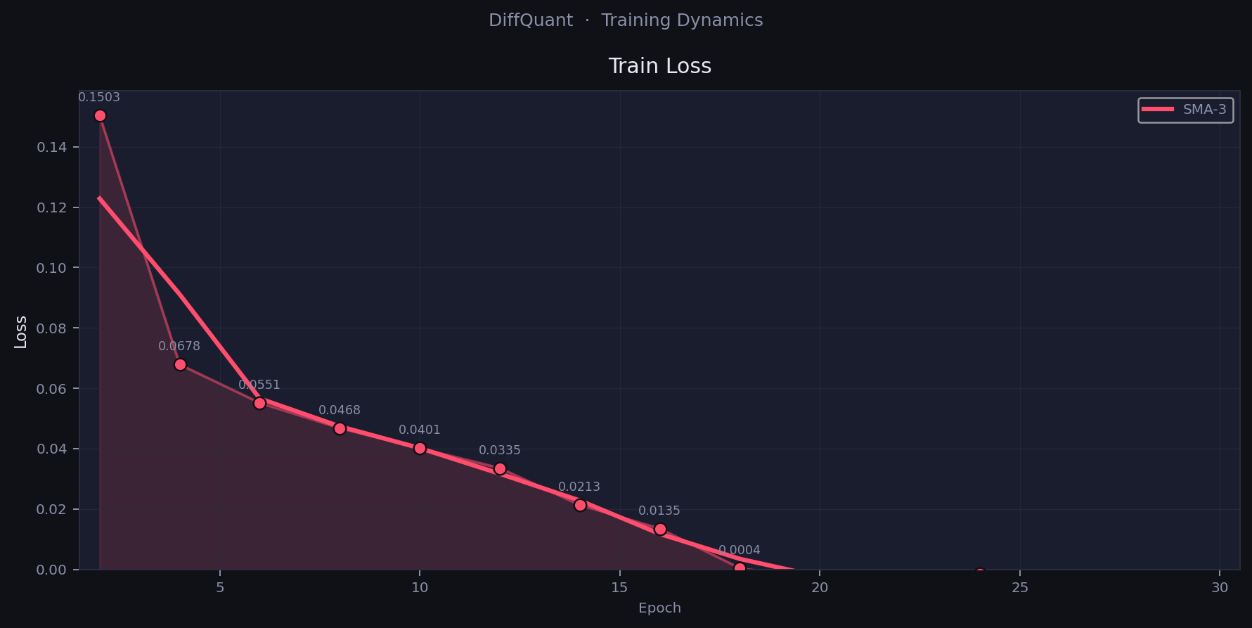
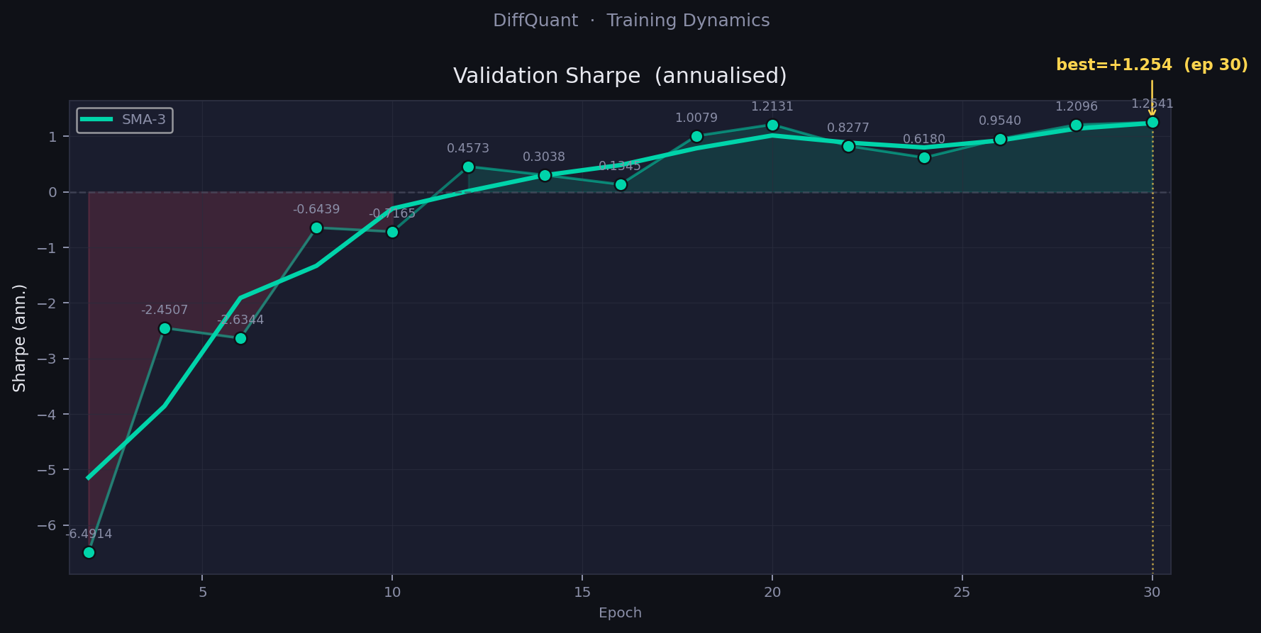
| Epoch | Val Sharpe | Val Return | Flat% | Turnover/bar | |---|---|---|---|---| | 2 | −6.49 | −14.1% | 1.6% | 0.0335 | | 8 | −0.64 | −0.4% | 77.5% | 0.0003 | | 12 | +0.46 | +0.9% | 17.7% | 0.0035 | | 20 | +1.21 | +5.2% | 15.4% | 0.0101 | | 30 | +1.25 | +5.8% | 13.2% | 0.0135 |

Training passes through two sequential failure modes before settling into a workable regime: hyperactivity at epoch 2 (turnover = 0.0335, val Sharpe = −6.49), followed by flat collapse at epoch 8 (flat fraction = 77.5%). The hybrid loss resolves both. Best checkpoint saved at epoch 30, with val Sharpe still improving at run end, consistent with the hypothesis that the model had not yet fully converged.

Train Loss Val Sharpe

Val Flat Fraction Val Max Drawdown

Walk-forward evaluation

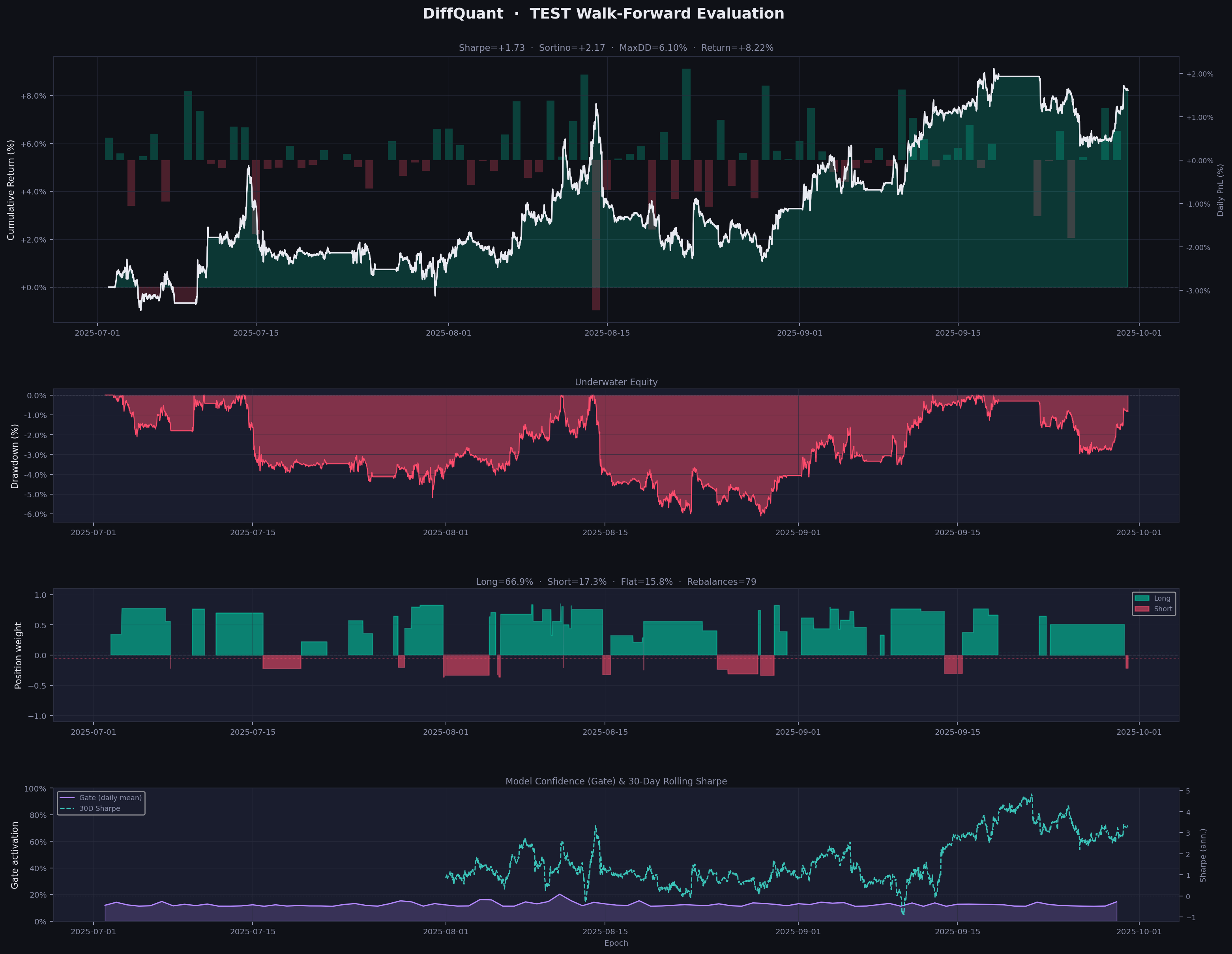
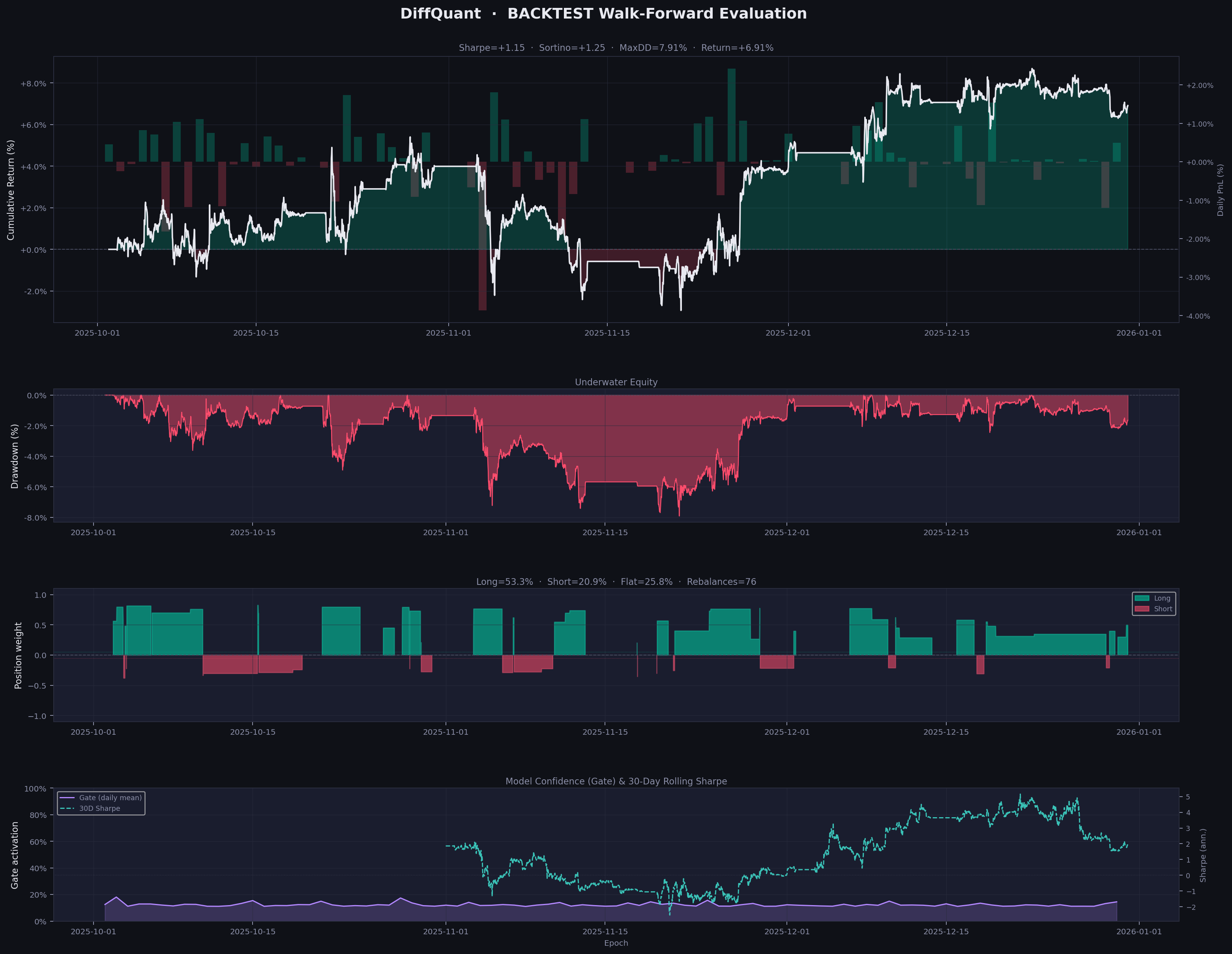
All evaluation uses the continuous walk-forward protocol, identical to live execution mechanics. No look-ahead, no episode resets.

Test — July–September 2025 (3 months, out-of-sample)

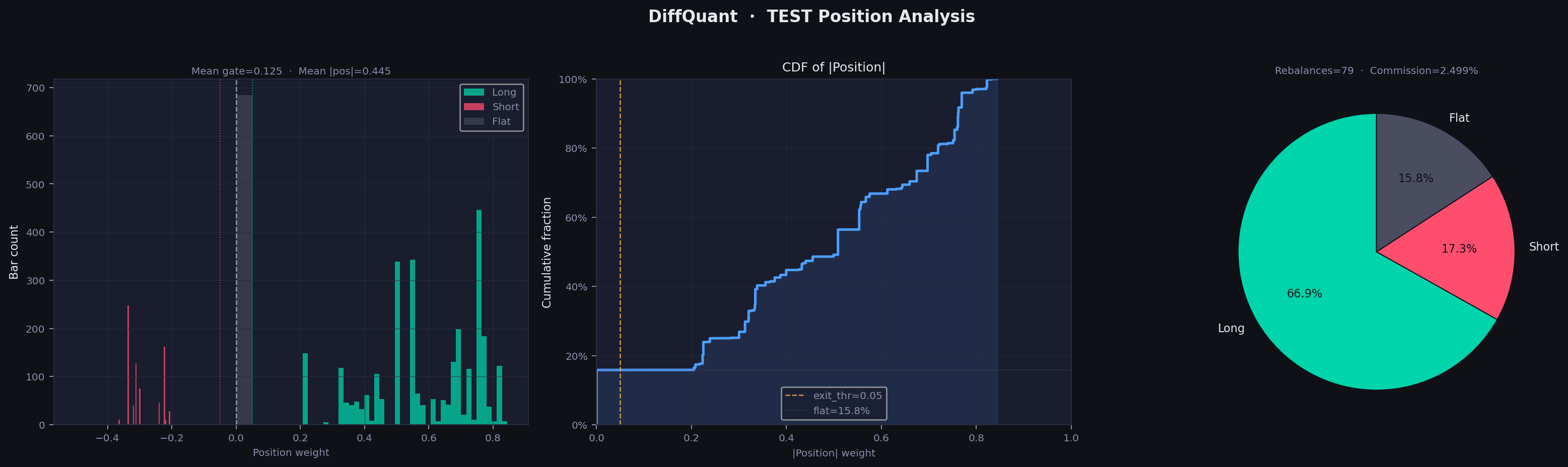
| Metric | Value | |---|---| | Sharpe (ann.) | +1.735 | | Sortino (ann.) | +2.173 | | Calmar | 1.346 | | Total return | +8.22% | | Max drawdown | 6.10% | | Commission paid | 2.50% | | Rebalances | 79 | | Long / Short / Flat | 66.9% / 17.3% / 15.8% |

Backtest — October–December 2025 (final hold-out, never touched during training)

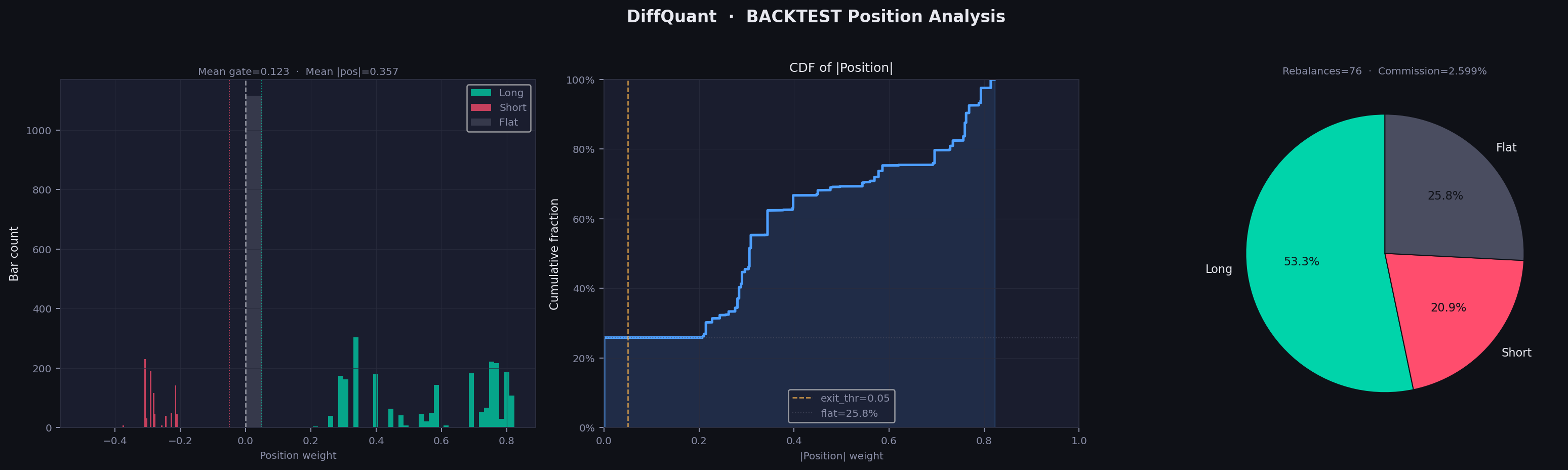
| Metric | Value | |---|---| | Sharpe (ann.) | +1.152 | | Sortino (ann.) | +1.250 | | Calmar | 0.874 | | Total return | +6.91% | | Max drawdown | 7.91% | | Commission paid | 2.60% | | Rebalances | 76 | | Long / Short / Flat | 53.3% / 20.9% / 25.8% |

Test Walk-Forward Evaluation

Backtest Walk-Forward Evaluation

Test Position Analysis Backtest Position Analysis

Key observations

Positive Sharpe on both held-out periods. Test (+1.73) and backtest (+1.15) are both positive. A single positive out-of-sample quarter can be coincidence; consistency across two non-overlapping quarters is a stronger signal.

Asymmetric learning from asymmetric data. The model was trained exclusively on Jan 2024 – Mar 2025, a predominantly bullish period for BTC. With mirroraugmentation=True, the training loop augments 50% of batches by inverting price returns, forcing symmetric long/short learning. Result: 17–21% short exposure in evaluation despite the long-biased training regime. Without augmentation, most prior configurations produced shortfraction close to zero.

Direction accuracy near 50% — and that is not a weakness. Long correct: 50.1–51.2%, short correct: 48.8–52.6%. The model's edge does not come from directional prediction accuracy but from asymmetric sizing: correctavgret (+0.065%) systematically exceeds incorrectavgret (−0.061%) in magnitude. The gate mechanism selectively suppresses low-confidence trades, improving the signal-to-noise ratio of executed positions.

Gate activation remains low. Mean gate ≈ 0.12–0.13. The model operates at partial exposure rather than full commitment, consistent with the conservative risk posture driven by lambdabias and flattarget regularization.

Limitations

Single asset. The pipeline trains one model per instrument. Multi-asset portfolio construction requires architectural extension.

Flat commission model. Costs are commissionrate + slippagerate applied uniformly. For positions large enough to move price, enable marketimpacteta in SimulatorConfig (quadratic Almgren-Chriss term).

Hyperparameter sensitivity. Loss weights, training window, feature composition, and learning rate interact non-trivially. This is not a plug-and-play recipe. It is a research framework that requires systematic tuning.

Limited statistical base. Two quarters is sufficient for a meaningful signal, but not for strong claims about statistical significance or long-term stability.

No live execution layer. There is no broker-facing execution module. Connecting to an exchange API requires additional engineering outside the current scope.

Roadmap

Multi-asset portfolio extension. The current architecture optimizes a single position. Extending to a portfolio requires a cross-asset attention layer and a portfolio-level Sharpe objective that accounts for position correlations. The differentiable simulator generalizes naturally: grosst = Σ weights{i,t-1} × ret_{i,t}.

Richer loss functions. The hybrid loss is a first approximation. Planned extensions include Calmar-based objectives, conditional drawdown penalties, and regime-aware loss weighting that adjusts λ values based on detected volatility regime.

Additional backbones. The LSTM encoder is implemented but not yet benchmarked against iTransformer under identical conditions. Planned ablations include PatchTST, Mamba, and linear attention variants.

Online data pipeline. A scheduled data collection layer (Binance WebSocket → local store → feature pipeline → model inference) to support paper trading and live monitoring.

Execution and risk layer. A broker-facing execution module with position sizing, stop-loss enforcement, and exchange connectivity. This is the final engineering step before any live deployment and is outside the current research scope.

Related work

**Buehler, H., Gonon, L., Teichmann, J., Wood, B. (2019). Deep Hedging. Quantitative Finance, 19(8), 1271–1291.** The foundational framework for training neural network policies end-to-end through a differentiable financial objective. DiffQuant adapts this paradigm from derivatives hedging to directional alpha generation.

**Liu, Y., Hu, T., Zhang, H., Wu, H., Wang, S., Ma, L., Long, M. (2024). iTransformer: Inverted Transformers Are Effective for Time Series Forecasting. ICLR 2024 Spotlight.** The backbone used in the primary DiffQuant experiment. Treats each feature channel as a token, capturing cross-variable dependencies rather than local temporal patterns.

**Moody, J., Saffell, M. (2001). Learning to trade via direct reinforcement. IEEE Transactions on Neural Networks, 12(4), 875–889.** The original formulation of direct PnL optimization as a training objective, predating the deep learning era. DiffQuant extends this to a fully differentiable end-to-end pipeline with modern architectures.

**Khubiev, K., Semenov, M., Podlipnova, I., Khubieva, D. (2026). Finance-Grounded Optimization For Algorithmic Trading. arXiv:2509.04541.** The closest parallel work: introduces Sharpe, PnL, and MaxDD as training loss functions for return prediction. DiffQuant differs by coupling the loss to a fully differentiable simulator, so gradient flows through the trading mechanics, not just through a prediction head.

Citation

@software{Kolesnikov2026diffquant,
  author  = {Kolesnikov, Yuriy},
  title   = {{DiffQuant}: End-to-End Differentiable Trading Pipeline},
  year    = {2026},
  url     = {https://github.com/YuriyKolesnikov/diffquant},
  version = {0.1.0}
}

MIT License. See LICENSE.

🔗 More in this category