Option Pricer

This is a Python project made to apply what I've learned about option pricing during my MSc in Finance.

References

• Hull, J. (2014) Options, Futures and Other Derivatives. 9th Edition
• A Black–Scholes user’s guide to the Bachelier model: https://arxiv.org/pdf/2104.08686.pdf
• Iacus, S.M. (2011) Option Pricing and Estimation of Financial Models with R

How to run

• Clone the repository or download it as ZIP file
• Run

  install -r requirements.txt

  (optional)
• Run

  .py [arguments]

Requirements

• numpy
• scipy
• matplotlib

Usage

• Supported underlying assets:

* Dividend and non-dividend paying stocks * Currencies * Commodities * Futures

| Argument | Description | |----------|---------------------------------------------------------------------------------------------------------------------------------------------------------------------------------------------------------------------------------------------------------------------------------------------------------------------| | h | Print help message | | m | Pricing Method

• Black-Scholes model, -m BS
• Bachelier model, -m BA
• Binomial Tree, -m BT
• Monte Carlo Simulation, -m MC

| | p | Product. The option type to price:

• European options: EUC (call), EUP (put)
• American options: USC (call), USP (put)
• Futures-style options: FSTYLEC (call), FSTYLEP (put)
• Bond options: BC (call), BP (put)

| | s | Spot Price | | f | Forward Price | | k | Strike Price | | r | Annualized Risk Free Rate | | rf | Annualized Foreign Risk Free Rate | | u | Annualized Storage Cost | | q | Annualized Dividend Yield | | d | Dividends. List of expected discrete dividends. e.g. three semi-annual dividends of 0.5$: -d 0.5 0.5 0.5 | | dt | Dividend Times. It refers to the times in which the dividends will be paid. In the example above we'll set: -dt 0.5 1 1.5 | | t | Time to Expiration. It can be expressed in different ways:

• Years, using only a float value e.g. -t 1
• Months, by adding "m" or "months" to a number e.g -t 12 m
• Weeks, by adding "w" or "weeks" e.g. -t 52 w
• Days, by adding "d" or "days" e.g. -t 252 d

| | vol | Annualized Log-Normal Volatility. The volatility used in Black-Scholes model and Binomial Trees. | | nvol | Annualized Normal Volatility. The volatility used in the Bachelier model.
If it isn't included when the Bachelier pricing model is selected, the tool will automatically convert log-normal volatility in normal volatility. | | b | Current Bond Cash Price | | i | PV of Bond's Income | | steps | Number of Steps. Number of steps to use in the binomial tree. | | print | Print the Binomial Tree | | greeks | Print the Values of Delta, Theta, Gamma, Vega and Rho | | n | Number of Simulations | | process | Underlying process

• Geometric Brownian Motion, -process GBM
• Variance-Gamma Process, -process VG
• Merton Jump Process, -process MJ

| | params | List of Process' Parameters. e.g. jumps' intensity, mean and standard deviation of jumps' distribution |

Examples

European option

A financial institution has just sold 1,000 seven-month European call options on the Japanese yen. Suppose that the spot exchange rate is 0.80 cent per yen, the exercise price is 0.81 cent per yen, the risk-free interest rate in the United States is 8% per annum, the risk-free interest rate in Japan is 5% per annum, and the volatility of the yen is 15% per annum. Calculate the delta, gamma, vega, theta, and rho of the financial institution’s position. Interpret each number

Black-Scholes

Input:

python main.py -p EUC -s 0.8 -k 0.81 -r 0.08 -rf 0.05 -vol 0.15 -t 7 m -greeks

Output:

INFO - pricers - Pricing using Black-Scholes
INFO - main - The option price is: 0.03741
INFO - main - The Greeks are: Theta -0.03989 | Delta 0.52493 | Gamma 4.20593 | Vega 0.23553 | Rho 0.22315

Bachelier

Input:

python main.py -p EUC -s 0.8 -k 0.81 -r 0.08 -rf 0.05 -vol 0.15 -t 7 m -m BA

Output:

INFO - pricers - Pricing using Bachelier
INFO - main - The option price is: 0.03751

Monte Carlo Simulation under GBM

Input:

python main.py -p EUC -s 0.8 -k 0.81 -r 0.08 -rf 0.05 -vol 0.15 -t 7 m -m MC -n 5000

Output:

INFO - pricers - Pricing using Monte Carlo Simulation
INFO - pricers - Pricing under Geometric Brownian Motion
INFO - main - The option price is: 0.03679

Monte Carlo Simulation under Variance-Gamma process

Input:

python main.py -p EUC -s 0.8 -k 0.81 -r 0.08 -rf 0.05 -vol 0.15 -t 7 m -m MC -n 5000 -process VG -params 0.02 1

Output:

INFO - pricers - Pricing using Monte Carlo Simulation
INFO - pricers - Pricing under Variance Gamma Process
INFO - main - The option price is: 0.04568

European option (dividend)

Consider a European call option on a stock when there are ex-dividend dates in two months and five months. The dividend on each ex-dividend date is expected to be $0.50. The current share price is $40, the exercise price is $40, the stock price volatility is 30% per annum, the risk-free rate of interest is 9% per annum, and the time to maturity is six months.

Input:

python main.py -p EUC -d 0.5 0.5 -dt 0.16667 0.41667 -s 40 -k 40 -vol 0.3 -r 0.09 -t 0.5

Output:

INFO - pricers - Pricing using Black-Scholes
INFO - main - The option price is: 3.67123

Futures-style option

The strike price of a futures option is 550 cents, the risk-free rate of interest is 3%, the volatility of the futures price is 20%, and the time to maturity of the option is 9 months. The futures price is 500 cents ... (d) What is the futures price for a futures style option if it is a call?

Input:

python main.py -p FSTYLEC -f 5 -k 5.5 -r 0.03 -vol 0.2 -t 0.75

Output:

INFO - pricers - Pricing using Black-Scholes
INFO - main - The option price is: 0.16564

Bond option

Use the Black’s model to value a one-year European put option on a 10-year bond. Assume that the current value of the bond is $125, the strike price is $110, the one-year risk-free interest rate is 10% per annum, the bond’s forward price volatility is 8% per annum, and the present value of the coupons to be paid during the life of the option is $10

Input:

python main.py -p BC -b 105 -i 34.968 -r 0.1 -t 4 -vol 0.02 -k 100

Output:

INFO - pricers - Pricing using Black-Scholes
INFO - main - The option price is: 3.19007

American Option

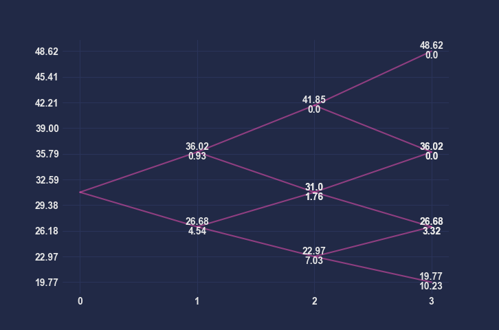
Three-step tree to value an American 9-month put option on a futures contract when the futures price is 31, strike price is 30, risk-free rate is 5%, and volatility is 30%

Input:

python main.py -m BT -steps 3 -p USP -f 31 -k 30 -r 0.05 -vol 0.3 -t 9 m -print

Output:

INFO - pricers - Pricing using Binomial Tree INFO - main - The option price is: 2.83564